如果你也在 怎样代写理论力学Theoretical Mechanics这个学科遇到相关的难题,请随时右上角联系我们的24/7代写客服。理论力学Theoretical Mechanics是一组密切相关的经典力学的替代公式。它是由许多科学家和数学家在18世纪及以后,在牛顿力学之后发展起来的。由于牛顿力学考虑的是运动的矢量,特别是系统中各组成部分的加速度、动量、力,因此由牛顿定律和欧拉定律所支配的力学的另一个名称是矢量力学。
理论力学Theoretical Mechanics使用代表系统整体的运动标量属性–通常是其总动能和势能–而不是牛顿对单个粒子的矢量力。运动方程是由标量通过一些关于标量变化的基本原理推导出来的。分析力学使用代表系统整体的运动标量属性–通常是其总动能和势能–而不是牛顿对单个粒子的矢量力。运动方程是由标量通过一些关于标量变化的基本原理推导出来的。
my-assignmentexpert™ 理论力学Theoretical Mechanics作业代写,免费提交作业要求, 满意后付款,成绩80\%以下全额退款,安全省心无顾虑。专业硕 博写手团队,所有订单可靠准时,保证 100% 原创。my-assignmentexpert™, 最高质量的理论力学Theoretical Mechanics作业代写,服务覆盖北美、欧洲、澳洲等 国家。 在代写价格方面,考虑到同学们的经济条件,在保障代写质量的前提下,我们为客户提供最合理的价格。 由于统计Statistics作业种类很多,同时其中的大部分作业在字数上都没有具体要求,因此理论力学Theoretical Mechanics作业代写的价格不固定。通常在经济学专家查看完作业要求之后会给出报价。作业难度和截止日期对价格也有很大的影响。
想知道您作业确定的价格吗? 免费下单以相关学科的专家能了解具体的要求之后在1-3个小时就提出价格。专家的 报价比上列的价格能便宜好几倍。
my-assignmentexpert™ 为您的留学生涯保驾护航 在物理physics作业代写方面已经树立了自己的口碑, 保证靠谱, 高质且原创的理论力学Theoretical Mechanics代写服务。我们的专家在物理physics代写方面经验极为丰富,各种理论力学Theoretical Mechanics相关的作业也就用不着 说。
我们提供的理论力学Theoretical Mechanics及其相关学科的代写,服务范围广, 其中包括但不限于:
物理代写|理论力学作业代写Theoretical Mechanics代考|Lagrange Equations
According to the considerations of the last section the most urgent objective must be to eliminate the in general not explicitly known constraint forces out of the equations of motion. Exactly that is the new aspect of the Lagrange mechanics compared to the Newtonian version. We start with the introduction of another important concept:
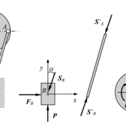
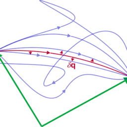
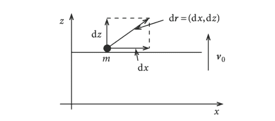
Definition 1.2.1 ‘virtual displacement’ $\delta \mathbf{r}{i}$ This is the arbitrary (virtual), infinitesimal coordinate change which has to be compatible with the constraints and is instantaneously executed. The latter means: $$ \delta t=0 . $$ The quantities $\delta \mathbf{r}{i}$ are not necessarily related to the real course of motion. They are therefore to be distinguished from the real displacements $d \mathbf{r}{i}$ in the time interval $d t$, in which the forces and the constraint forces can change: $$ \delta \longleftrightarrow \text { virtual } ; \quad d \longleftrightarrow \text { real } . $$ Mathematically we treat the symbol $\delta$ like the normal differential $d$. We elucidate the matter by a simple example (Fig. 1.10): Example: Particle in an Elevator The constraint (holonomic-rheonomic) has already been given in (1.8). A suitable generalized coordinate is $q=x$. But then it holds because of $\delta t=0$ : real displacement: $\quad d \mathbf{r}=(d x, d z)=\left(d q, v{0} d t\right)$,
virtual displacement $\quad \delta \mathbf{r}=(\delta x, \delta z)=(\delta q, 0)$.
Definition 1.2.2 Virtual work
$$
\delta W_{i}=-\mathbf{F}{i} \cdot \delta \mathbf{r}{i}
$$
$\mathbf{F}{i}$ is the force acting on particle $i$ : $$ \mathbf{F}{i}=\mathbf{K}{i}+\mathbf{Z}{i}=m_{i} \ddot{\mathbf{r}}{i} $$ $\mathbf{K}{i}$ is the driving force acting on the mass point which is somewhat limited in its mobility because of certain constraints. $\mathbf{Z}_{i}$ is the constraint force.
物理代写|理论力学作业代写Theoretical Mechanics代考|Simple Applications
In this section we want to demonstrate and practice extensively the algorithm which is usually applied for the solution of mechanical problems by exploiting the Lagrange equations. Throughout the following considerations we will presume holonomic constraints, conservative forces
The solution method then consists of six sub-steps:
- Formulate the constraints.
- Choose proper generalized coordinates $\mathbf{q}$.
- Find the transformation formulas.
- Write down the Lagrangian function $L=T-V=L(\mathbf{q}, \dot{\mathbf{q}}, t)$.
- Derive and solve the Lagrange equation (1.36).
- Back transformation to the original, ‘illustrative’ coordinates.
We want to exercise this procedure with some typical examples.
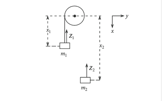
(1) Atwood’s Free-Fall Machine
It is about a conservative system with holonomic-scleronomic constraints (Fig. 1.15):
$$
\begin{aligned}
x_{1}+x_{2} &=l-\pi R=\text { const } \
y_{1} &=z_{1}=z_{2}=0, \quad y_{2}=2 R
\end{aligned}
$$
There thus remains
$$
S=6-5=1
$$
物理代写|理论力学作业代写THEORETICAL MECHANICS代考|Generalized Potentials
The simple examples of the last section presume the validity of the Lagrange equations in the form (1.36). They concern conservative systems with holonomic constraints. For non-conservative systems, but with holonomic constraints, instead of that, the starting point must be (1.33):
$$
\frac{d}{d t} \frac{\partial T}{\partial \dot{q}{j}}-\frac{\partial T}{\partial q{j}}=Q_{j}, \quad j=1,2, \ldots, S .
$$
However, we come to formally unchanged Lagrange equations for the so-called Generalized potentials
$$
U=U\left(q_{1}, \ldots, q_{S}, \dot{q}{1}, \ldots, \dot{q}{S}, t\right)
$$
if the generalized forces $Q_{j}$ are derivable from $U$ by:
$$
Q_{j}=\frac{d}{d t} \frac{\partial U}{\partial \dot{q}{j}}-\frac{\partial U}{\partial q{j}}, \quad j=1,2, \ldots, S
$$
The first term on the right-hand side is new compared to the case of a conservative system. For the
Generalized Lagrangian function
$$
L=T-U
$$
the equations of motion are obviously valid, because of (1.71), in the formally unchanged version (1.36). On the other hand, the requirement (1.71) appears to be very special. However, there does exist a very important application example:
Charged particle in an electromagnetic field
In Vol. 3 we will learn that a particle with charge $\bar{q}$ which moves with the velocity $\mathbf{v}$ in an electromagnetic field (electrical field $\mathbf{E}$, magnetic induction $\mathbf{B}$ ) experiences the so-called ‘Lorentz force’
$$
\mathbf{F}=\bar{q}[\mathbf{E}+(\mathbf{v} \times \mathbf{B})]
$$
理论力学代写
物理代写|理论力学作业代写THEORETICAL MECHANICS代考|LAGRANGE EQUATIONS
根据上一节的考虑,最紧迫的目标必须是从运动方程中消除通常不明确已知的约束力。与牛顿版本相比,这正是拉格朗日力学的新方面。我们先介绍另一个重要的概念:
定义 1.2.1 ‘虚位移”virtual displacement’ $\delta \mathbf{r}{i}$ This is the arbitrary (virtual), infinitesimal coordinate change which has to be compatible with the constraints and is instantaneously executed. The latter means: $$ \delta t=0 . $$ The quantities $\delta \mathbf{r}{i}$ are not necessarily related to the real course of motion. They are therefore to be distinguished from the real displacements $d \mathbf{r}{i}$ in the time interval $d t$, in which the forces and the constraint forces can change: $$ \delta \longleftrightarrow \text { virtual } ; \quad d \longleftrightarrow \text { real } . $$ Mathematically we treat the symbol $\delta$ like the normal differential $d$. We elucidate the matter by a simple example (Fig. 1.10): Example: Particle in an Elevator The constraint (holonomic-rheonomic) has already been given in (1.8). A suitable generalized coordinate is $q=x$. But then it holds because of $\delta t=0$ : real displacement: $\quad d \mathbf{r}=(d x, d z)=\left(d q, v{0} d t\right)$,
virtual displacement $\quad \delta \mathbf{r}=(\delta x, \delta z)=(\delta q, 0)$.
Definition 1.2.2 Virtual work
$$
\delta W_{i}=-\mathbf{F}{i} \cdot \delta \mathbf{r}{i}
$$
$\mathbf{F}{i}$ is the force acting on particle $i$ : $$ \mathbf{F}{i}=\mathbf{K}{i}+\mathbf{Z}{i}=m_{i} \ddot{\mathbf{r}}{i} $$ $\mathbf{K}{i}$ is the driving force acting on the mass point which is somewhat limited in its mobility because of certain constraints. $\mathbf{Z}_{i}$ 是约束力。
物理代写|理论力学作业代写THEORETICAL MECHANICS代考|SIMPLE APPLICATIONS
在本节中,我们将演示和广泛实践通常通过利用拉格朗日方程来解决机械问题的算法。在以下考虑中,我们将假定完整约束、保守力求
解方法包括六个子步骤:
- 制定约束。
- 选择适当的广义坐标q.
- 找到转换公式。
- 写出拉格朗日函数大号=吨−五=大号(q,q˙,吨).
- 推导和求解拉格朗日方程1.36.
- 返回到原始“说明性”坐标的转换。
我们想用一些典型的例子来练习这个过程。
1阿特伍德的自由落体机器
它是关于具有完整-硬化约束的保守系统F一世G.1.15:
X1+X2=一世−圆周率R= 常量 是1=和1=和2=0,是2=2R
因此剩下
小号=6−5=1
物理代写|理论力学作业代写THEORETICAL MECHANICS代考|GENERALIZED POTENTIALS
上一节的简单例子假定了拉格朗日方程的有效性,形式为1.36. 他们关注具有完整约束的保守系统。对于非保守系统,但具有完整约束,而不是那样,起点必须是1.33:
$$
\frac{d}{d t} \frac{\partial T}{\partial \dot{q}{j}}-\frac{\partial T}{\partial q{j}}=Q_{j}, \quad j=1,2, \ldots, S .
$$
However, we come to formally unchanged Lagrange equations for the so-called Generalized potentials
$$
U=U\left(q_{1}, \ldots, q_{S}, \dot{q}{1}, \ldots, \dot{q}{S}, t\right)
$$
if the generalized forces $Q_{j}$ are derivable from $U$ by:
$$
Q_{j}=\frac{d}{d t} \frac{\partial U}{\partial \dot{q}{j}}-\frac{\partial U}{\partial q{j}}, \quad j=1,2, \ldots, S
$$
The first term on the right-hand side is new compared to the case of a conservative system. For the
Generalized Lagrangian function
$$
L=T-U
$$
the equations of motion are obviously valid, because of (1.71), in the formally unchanged version (1.36). On the other hand, the requirement (1.71) appears to be very special. However, there does exist a very important application example:
Charged particle in an electromagnetic field
In Vol. 3 we will learn that a particle with charge $\bar{q}$ which moves with the velocity $\mathbf{v}$ in an electromagnetic field (electrical field $\mathbf{E}$, magnetic induction $\mathbf{B}$ ) experiences the so-called ‘Lorentz force’
$$
\mathbf{F}=\bar{q}[\mathbf{E}+(\mathbf{v} \times \mathbf{B})]
$$

物理代写|理论力学作业代写Theoretical Mechanics代考 请认准UprivateTA™. UprivateTA™为您的留学生涯保驾护航。