如果你也在 怎样代写理论力学Theoretical Mechanics这个学科遇到相关的难题,请随时右上角联系我们的24/7代写客服。理论力学Theoretical Mechanics是一组密切相关的经典力学的替代公式。它是由许多科学家和数学家在18世纪及以后,在牛顿力学之后发展起来的。由于牛顿力学考虑的是运动的矢量,特别是系统中各组成部分的加速度、动量、力,因此由牛顿定律和欧拉定律所支配的力学的另一个名称是矢量力学。
理论力学Theoretical Mechanics使用代表系统整体的运动标量属性–通常是其总动能和势能–而不是牛顿对单个粒子的矢量力。运动方程是由标量通过一些关于标量变化的基本原理推导出来的。分析力学使用代表系统整体的运动标量属性–通常是其总动能和势能–而不是牛顿对单个粒子的矢量力。运动方程是由标量通过一些关于标量变化的基本原理推导出来的。
my-assignmentexpert™ 理论力学Theoretical Mechanics作业代写,免费提交作业要求, 满意后付款,成绩80\%以下全额退款,安全省心无顾虑。专业硕 博写手团队,所有订单可靠准时,保证 100% 原创。my-assignmentexpert™, 最高质量的理论力学Theoretical Mechanics作业代写,服务覆盖北美、欧洲、澳洲等 国家。 在代写价格方面,考虑到同学们的经济条件,在保障代写质量的前提下,我们为客户提供最合理的价格。 由于统计Statistics作业种类很多,同时其中的大部分作业在字数上都没有具体要求,因此理论力学Theoretical Mechanics作业代写的价格不固定。通常在经济学专家查看完作业要求之后会给出报价。作业难度和截止日期对价格也有很大的影响。
想知道您作业确定的价格吗? 免费下单以相关学科的专家能了解具体的要求之后在1-3个小时就提出价格。专家的 报价比上列的价格能便宜好几倍。
my-assignmentexpert™ 为您的留学生涯保驾护航 在物理physics作业代写方面已经树立了自己的口碑, 保证靠谱, 高质且原创的理论力学Theoretical Mechanics代写服务。我们的专家在物理physics代写方面经验极为丰富,各种理论力学Theoretical Mechanics相关的作业也就用不着 说。
我们提供的理论力学Theoretical Mechanics及其相关学科的代写,服务范围广, 其中包括但不限于:
物理代写|理论力学作业代写Theoretical Mechanics代考|Formulation of the Principle
For a better understanding of the integral principle let us recall once more two previous definitions. We understand by the
configuration space
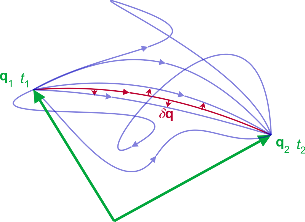
the $S$-dimensional space the axes of which are given by the generalized coordinates $q_{1}, \ldots, q_{s}$. Each point of the configuration space specifies a possible state of the total system. There need not necessarily exist a compelling link between the configuration space and the three-dimensional physical space. The curve in the configuration space which the system runs through in the course of time is called configuration path: $\quad \mathbf{q}(t)=\left(q_{1}(t), \ldots, q_{S}(t)\right)$.
On this path the system moves as a whole. Therefore, it may be that the configuration path does not have the slightest similarity to the actual particle paths.
We restrict the following considerations at first to
holonomic, conservative systems.
Generalizations are discussed later in the text. If one inserts into the Lagrangian the configuration path $\mathbf{q}(t)$ and its time-derivative $\dot{\mathbf{q}}(t)$ then $L$ becomes a pure timefunction:
$$
L(\mathbf{q}(t), \dot{\mathbf{q}}(t), t) \equiv \widetilde{L}(t)
$$
We define:
$$
S{\mathbf{q}(t)}=\int_{t_{1}}^{t_{2}} \widetilde{L}(t) d t
$$
$S$ has the dimension of ‘action'(=energy $\times$ time) and is dependent on the times $t_{1}$, $t_{2}$ as well as on the path $\mathbf{q}(t)$. For fixed $t_{1}, t_{2}$ to each path $\mathbf{q}(t)$ a pure number $S{\mathbf{q}(t)}$ is ascribed. This is called a ‘functional’. To each point of the system’s path a manifold of virtual displacements $\delta \mathbf{q}$ exists which along the path form something like a continuum. One can now consider virtual displacements to be composed in such a way that they, on their own part, represent a continuously differentiable ‘variational orbit’. Such a composition of virtual displacements may be done in totally different manners so that a full manifold of variational orbits can be found.
物理代写|理论力学作业代写Theoretical Mechanics代考|Elements of the Calculus of Variations
How can we exploit in practice the Hamilton’s principle, i.e. how can we infer the ‘stationary’ path from the action functional $S{\mathbf{q}(t)}$ ? The task to find the curve for which a definite line integral becomes extremal represents a typical
variational problem
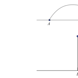
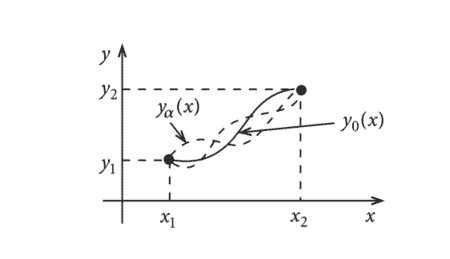
At first we will outline the main features for a one-dimensional problem (Fig. 1.44).
We define as
‘competing ensemble $\mathbf{M}$ ‘
$M \equiv\left{y(x)\right.$; at least twofold differentiable with $y\left(x_{1}\right)=y_{1}$ and $\left.y\left(x_{2}\right)=y_{2}\right}$, and on this the functional:
$$
J{y(x)}=\int_{x_{1}}^{x_{2}} f\left(x, y, y^{\prime}\right) d x=\int_{x_{1}}^{x_{2}} \tilde{f}(x) d x
$$
where $y^{\prime}=d y / d x$, while $f(u, v, w)$ represents a differentiable function with continuous partial derivatives.
物理代写|理论力学作业代写THEORETICAL MECHANICS代考|Lagrange Equations
We have first to generalize the variational calculus to more than one variable. From the requirement
$$
\delta J=\delta \int_{x_{1}}^{x_{2}} d x f\left(x, y_{1}(x), \ldots, y_{S}(x), y_{1}^{\prime}(x), \ldots, y_{S}^{\prime}(x)\right) \stackrel{!}{=} 0
$$
the extremal (stationary) path $\mathbf{y}(x)=\left(y_{1}(x), \ldots, y_{S}(x)\right)$ is to be derived. For each single component we define a ‘competing ensemble’ $M_{i}$ by:
$M_{i}=\left{y_{i}(x)\right.$; at least two times differentiable with $y_{i}\left(x_{1}\right)=y_{i 1}$ and $\left.y_{i}\left(x_{2}\right)=y_{i 2}\right}$.
We use here again a parameter representation for the component function $y_{i}(x)$ :
$$
y_{i \alpha}(x)=y_{i 0}(x)+\gamma_{i \alpha}(x), \quad i=1,2, \ldots, S
$$
$y_{i 0}(x)$ are here the solutions of the extreme-value problem and $\gamma_{i \alpha}(x)$ ‘almost arbitrary’, but sufficiently often differentiable functions with
$$
\begin{aligned}
\gamma_{i \alpha}\left(x_{1}\right)=\gamma_{i \alpha}\left(x_{2}\right)=0 & \forall \alpha, i \
\gamma_{i \alpha=0}(x)=0 & \forall x, i
\end{aligned}
$$
The variations $\delta y_{i}$ of the path components,
$$
\delta y_{i}=\left(\frac{\partial y_{i \alpha}}{\partial \alpha}\right){x, \alpha=0} d \alpha $$ and the variation $\delta J$ of the functional, $$ \delta J=\left(\frac{d J(\alpha)}{d \alpha}\right){\alpha=0} d \alpha=\int_{x_{1}}^{x_{2}} d x \sum_{i=1}^{S}\left(\frac{\partial f}{\partial y_{i}} \frac{\partial y_{i}}{\partial \alpha}+\frac{\partial f}{\partial y_{i}^{\prime}} \frac{\partial y_{i}^{\prime}}{\partial \alpha}\right){\alpha=0} d \alpha $$ are defined analogously to the special cases $(S=1)$ (1.129) and (1.130), respectively. A partial integration of the second term in (1.145) yields: $$ \int{x_{1}}^{x_{2}} d x \frac{\partial f}{\partial y_{i}^{\prime}} \frac{\partial y_{i}^{\prime}}{\partial \alpha}=\int_{x_{1}}^{x_{2}} d x \frac{\partial f}{\partial y_{i}^{\prime}} \frac{d}{d x} \frac{\partial y_{i}}{\partial \alpha}=\left.\frac{\partial f}{\partial y_{i}^{\prime}} \frac{\partial y_{i}}{\partial \alpha}\right|{x{1}} ^{x_{2}}-\int_{x_{1}}^{x_{2}} d x\left(\frac{d}{d x} \frac{\partial f}{\partial y_{i}^{\prime}}\right) \frac{\partial y_{i}}{\partial \alpha}
$$
The first summand disappears because of $(1.143)$ so that it remains in (1.145):
$$
\delta J=\int_{x_{1}}^{x_{2}} d x \sum_{i=1}^{S}\left(\frac{\partial f}{\partial y_{i}}-\frac{d}{d x} \frac{\partial f}{\partial y_{i}^{\prime}}\right) \delta y_{i} \stackrel{!}{=} 0
$$
理论力学代写
物理代写|理论力学作业代写THEORETICAL MECHANICS代考|FORMULATION OF THE PRINCIPLE
为了更好地理解积分原理,让我们再次回顾一下前面的两个定义。
我们通过配置空间
来理解小号维空间,其轴由广义坐标给出q1,…,qs. 配置空间的每个点都指定了整个系统的可能状态。配置空间和三维物理空间之间不一定存在强制链接。系统在配置空间中随时间运行的曲线称为配置路径:q(吨)=(q1(吨),…,q小号(吨)).
在这条路径上,系统作为一个整体移动。因此,配置路径可能与实际粒子路径没有丝毫相似之处。
我们首先将以下考虑限制在
完整的保守系统上。
泛化将在本文后面讨论。如果将配置路径插入拉格朗日q(吨)及其时间导数q˙(吨)然后大号变成纯时间函数:
大号(q(吨),q˙(吨),吨)≡大号~(吨)
我们定义:
小号q(吨)=∫吨1吨2大号~(吨)d吨
小号具有“行动”的维度=和n和rG是$×$吨一世米和并且取决于时代吨1,吨2以及在路上q(吨). 对于固定吨1,吨2到每条路径q(吨)一个纯数小号q(吨)归于。这被称为“功能性”。对于系统路径的每个点,虚拟位移的流形dq存在,沿着路径形成类似连续体的东西。现在可以考虑以这样一种方式组合虚拟位移,即它们本身代表一个连续可微的“变分轨道”。这种虚拟位移的组合可以以完全不同的方式完成,以便可以找到变分轨道的完整流形。
物理代写|理论力学作业代写THEORETICAL MECHANICS代考|ELEMENTS OF THE CALCULUS OF VARIATIONS
我们如何在实践中利用汉密尔顿原理,即我们如何从动作泛函中推断出“平稳”路径小号q(吨)? 找到一个确定的线积分变为极值的曲线的任务代表了一个典型的
变分问题
首先,我们将概述一维问题的主要特征F一世G.1.44.
我们将其定义为
“竞争合奏”米‘
M \equiv\left{y(x)\right.$; 至少可以用 $y\left(x_{1}\right)=y_{1}$ 和 $\left.y\left(x_{2}\right)=y_{2}\right} 进行二次微分M \equiv\left{y(x)\right.$; 至少可以用 $y\left(x_{1}\right)=y_{1}$ 和 $\left.y\left(x_{2}\right)=y_{2}\right} 进行二次微分,并在此功能:
Ĵ是(X)=∫X1X2F(X,是,是′)dX=∫X1X2F~(X)dX
在哪里是′=d是/dX, 尽管F(你,v,在)表示具有连续偏导数的可微函数.
物理代写|理论力学作业代写THEORETICAL MECHANICS代考|LAGRANGE EQUATIONS
我们必须首先将变分演算推广到多个变量。从要求
dĴ=d∫X1X2dXF(X,是1(X),…,是小号(X),是1′(X),…,是小号′(X))=!0
the extremal (stationary) path $\mathbf{y}(x)=\left(y_{1}(x), \ldots, y_{S}(x)\right)$ is to be derived. For each single component we define a ‘competing ensemble’ $M_{i}$ by:
$M_{i}=\left{y_{i}(x)\right.$; at least two times differentiable with $y_{i}\left(x_{1}\right)=y_{i 1}$ and $\left.y_{i}\left(x_{2}\right)=y_{i 2}\right}$.
We use here again a parameter representation for the component function $y_{i}(x)$ :
$$
y_{i \alpha}(x)=y_{i 0}(x)+\gamma_{i \alpha}(x), \quad i=1,2, \ldots, S
$$
$y_{i 0}(x)$ are here the solutions of the extreme-value problem and $\gamma_{i \alpha}(x)$ ‘almost arbitrary’, but sufficiently often differentiable functions with
$$
\begin{aligned}
\gamma_{i \alpha}\left(x_{1}\right)=\gamma_{i \alpha}\left(x_{2}\right)=0 & \forall \alpha, i \
\gamma_{i \alpha=0}(x)=0 & \forall x, i
\end{aligned}
$$
The variations $\delta y_{i}$ of the path components,
$$
\delta y_{i}=\left(\frac{\partial y_{i \alpha}}{\partial \alpha}\right){x, \alpha=0} d \alpha $$ and the variation $\delta J$ of the functional, $$ \delta J=\left(\frac{d J(\alpha)}{d \alpha}\right){\alpha=0} d \alpha=\int_{x_{1}}^{x_{2}} d x \sum_{i=1}^{S}\left(\frac{\partial f}{\partial y_{i}} \frac{\partial y_{i}}{\partial \alpha}+\frac{\partial f}{\partial y_{i}^{\prime}} \frac{\partial y_{i}^{\prime}}{\partial \alpha}\right){\alpha=0} d \alpha $$ are defined analogously to the special cases $(S=1)$ (1.129) and (1.130), respectively. A partial integration of the second term in (1.145) yields: $$ \int{x_{1}}^{x_{2}} d x \frac{\partial f}{\partial y_{i}^{\prime}} \frac{\partial y_{i}^{\prime}}{\partial \alpha}=\int_{x_{1}}^{x_{2}} d x \frac{\partial f}{\partial y_{i}^{\prime}} \frac{d}{d x} \frac{\partial y_{i}}{\partial \alpha}=\left.\frac{\partial f}{\partial y_{i}^{\prime}} \frac{\partial y_{i}}{\partial \alpha}\right|{x{1}} ^{x_{2}}-\int_{x_{1}}^{x_{2}} d x\left(\frac{d}{d x} \frac{\partial f}{\partial y_{i}^{\prime}}\right) \frac{\partial y_{i}}{\partial \alpha}
$$
The first summand disappears because of $(1.143)$ so that it remains in (1.145):
$$
\delta J=\int_{x_{1}}^{x_{2}} d x \sum_{i=1}^{S}\left(\frac{\partial f}{\partial y_{i}}-\frac{d}{d x} \frac{\partial f}{\partial y_{i}^{\prime}}\right) \delta y_{i} \stackrel{!}{=} 0
$$
$$

物理代写|理论力学作业代写Theoretical Mechanics代考 请认准UprivateTA™. UprivateTA™为您的留学生涯保驾护航。