如果你也在 怎样代写电动力学electrodynamics这个学科遇到相关的难题,请随时右上角联系我们的24/7代写客服。电动力学electrodynamics是物理学的一个分支,涉及到对电磁力的研究,这是一种发生在带电粒子之间的物理作用。电磁力是由电场和磁场组成的电磁场所承载的,它是诸如光这样的电磁辐射的原因。它与强相互作用、弱相互作用和引力一起,是自然界的四种基本相互作用(通常称为力)之一。
电动力学electrodynamics电磁现象是以电磁力来定义的,有时也称为洛伦兹力,它包括电和磁,是同一现象的不同表现形式。电磁力在决定日常生活中遇到的大多数物体的内部属性方面起着重要作用。原子核和其轨道电子之间的电磁吸引力将原子固定在一起。电磁力负责原子之间形成分子的化学键,以及分子间的力量。电磁力支配着所有的化学过程,这些过程是由相邻原子的电子之间的相互作用产生的。电磁学在现代技术中应用非常广泛,电磁理论是电力工程和电子学包括数字技术的基础。
my-assignmentexpert™ 电动力学electrodynamics作业代写,免费提交作业要求, 满意后付款,成绩80\%以下全额退款,安全省心无顾虑。专业硕 博写手团队,所有订单可靠准时,保证 100% 原创。my-assignmentexpert™, 最高质量的电动力学electrodynamics作业代写,服务覆盖北美、欧洲、澳洲等 国家。 在代写价格方面,考虑到同学们的经济条件,在保障代写质量的前提下,我们为客户提供最合理的价格。 由于统计Statistics作业种类很多,同时其中的大部分作业在字数上都没有具体要求,因此电动力学electrodynamics作业代写的价格不固定。通常在经济学专家查看完作业要求之后会给出报价。作业难度和截止日期对价格也有很大的影响。
想知道您作业确定的价格吗? 免费下单以相关学科的专家能了解具体的要求之后在1-3个小时就提出价格。专家的 报价比上列的价格能便宜好几倍。
my-assignmentexpert™ 为您的留学生涯保驾护航 在物理physics作业代写方面已经树立了自己的口碑, 保证靠谱, 高质且原创的电动力学electrodynamics代写服务。我们的专家在物理physics代写方面经验极为丰富,各种电动力学electrodynamics相关的作业也就用不着 说。
我们提供的电动力学electrodynamics及其相关学科的代写,服务范围广, 其中包括但不限于:
物理代写|电动力学作业代electrodynamics代考|Electric Multipole Expansion
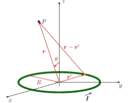
The scalar potential $\Phi(\mathbf{x})$ due to a charge distribution $\rho\left(\mathbf{x}^{\prime}\right)$ is given by
$$
\Phi(\mathbf{x})=\int \frac{\rho\left(\mathbf{x}^{\prime}\right)}{\left|\mathbf{x}-\mathbf{x}^{\prime}\right|} d^{3} x^{\prime}
$$
Far away from the localized charge distribution, the observer will see the total charge $Q$ of the distribution, effectively as a point charge, and the potential will fall off as inverse of the distance between the charge and the observation point. However, even if the total charge $Q$ is zero, the scalar potential at $\mathbf{x}$ outside the charge distribution may not be zero. It turns out that $\Phi(\mathbf{x})$ can be expressed in terms of ‘multipole moments’ dictated by the geometry of the charge distribution. We note that $|\mathbf{x}|=r$ and $\left|\mathbf{x}^{\prime}\right|=r^{\prime}$. Then,
$$
\begin{aligned}
\frac{1}{\left|\mathbf{x}-\mathbf{x}^{\prime}\right|} &=\left(\mathbf{x}^{2}+\mathbf{x}^{\prime 2}-2 \mathbf{x} \cdot \mathbf{x}^{\prime}\right)^{-1 / 2} \
&=\frac{1}{r}\left[1+\left(\frac{r^{\prime}}{r}\right)^{2}-\frac{2}{r^{2}} \sum_{i} x_{i} x_{i}^{\prime}\right]^{-\frac{1}{2}} .
\end{aligned}
$$
For points outside the charge distribution, $r^{\prime} \ll r$, we can use the binomial expansion
$$
(1+\varepsilon)^{-\frac{1}{2}}=\sum_{n=0}^{\infty}(-1)^{n} \frac{(2 n-1) ! !}{n ! 2^{n}} \varepsilon^{n},
$$
where $\varepsilon=\left(\frac{r^{\prime}}{r}\right)^{2}-\frac{2}{r^{2}} \sum_{i} x_{i} x_{i}^{\prime}$. Therefore,
$$
\begin{aligned}
\frac{1}{\left|\mathbf{x}-\mathbf{x}^{\prime}\right|} &=\frac{1}{r} \sum_{n=0}^{\infty}(-1)^{n} \frac{(2 n-1) ! !}{n ! 2^{n}}\left[\left(\frac{r^{\prime}}{r}\right)^{2}-\frac{2}{r^{2}} \sum_{i} x_{i} x_{i}^{\prime}\right] \
&=\sum_{n=0}^{\infty} \frac{(-1)^{n}}{r^{2 n+1}} \frac{(2 n-1) ! !}{n ! 2^{n}}\left[r^{\prime 2}-2 \sum_{i} x_{i} x_{i}^{\prime}\right]^{n} .
\end{aligned}
$$
物理代写|电动力学作业代electrodynamics代考|The Electric Dipole Moment
The monopole moment $q$ is the net charge of the distribution. Since the monopole term in the potential falls off as $\frac{1}{r}$, it will dominate the potential at large $r$, whenever $q$ is non-zero. The electric dipole moment $\mathbf{p}$ is non-zero for any spatially extended charge distribution where the ‘centers’ of the positively charged and negatively charged components are displaced with respect to each other. A given charge distribution in a macroscopic medium possesses ‘permanent electric dipole moment’ when $\mathbf{p}$ is non-zero in the absence of the electric field. We could also have a scenario where the electric dipole moments in a medium are produced by the external electric field. These are called ‘induced dipole moments’. Regardless of the physical origin of the electric dipole moment, $\Phi_{\mathrm{dip}}=\frac{\mathbf{p} \cdot \mathbf{x}}{r^{3}}$ describes the true potential far from the distribution.
In general, the multipole moments are dependent on the choice of origin of the coordinate system. This can be easily understood using a simple example. Take a point charge $q$ and calculate the potential anywhere by shifting the origin of the coordinate-ordinate system away from the location of the charge. You will see all sorts of multipole potentials appearing in the expansion! The monopole moment $q$ itself is a scalar and as such invariant under coordinate transformation. The dipole moment, on the other hand, is dependent on the choice of the origin so long as the net charge is non-zero. This can be proven with a simple argument. Let $\mathbf{p}^{\prime}$ be the ‘new’ dipole moment when the origin is shifted by $\delta$ so that in the ‘new’ coordinate system, $\mathbf{x}^{\prime \prime}=\mathbf{x}^{\prime}+\delta$ and $\rho\left(\mathbf{x}^{\prime \prime}\right)=\rho\left(\mathbf{x}^{\prime}\right)$. Then, $\mathbf{p}^{\prime}=\int \mathbf{x}^{\prime \prime} \rho\left(\mathbf{x}^{\prime \prime}\right) d^{3} x^{\prime \prime}=$ $\int\left(\mathbf{x}^{\prime}+\delta\right) \rho\left(\mathbf{x}^{\prime}\right) d^{3} x^{\prime}=\mathbf{p}+\delta \int \rho\left(\mathbf{x}^{\prime}\right) d^{3} x^{\prime}=\mathbf{p}+q \delta$. Clearly, $\mathbf{p}=\mathbf{p}^{\prime}$ only when $q=$ 0 .
As an illustration, let us calculate the dipole moment of two point charges $\pm q$ placed at $\mathbf{x}^{\prime}=\pm \frac{1}{2} \mathbf{d}$, respectively. The charge density can be expressed as $\rho\left(\mathbf{x}^{\prime}\right)=$ $q \delta\left(\mathbf{x}^{\prime}-\frac{1}{2} \mathbf{d}\right)-q \delta\left(\mathbf{x}^{\prime}+\frac{1}{2} \mathbf{d}\right)$. Using Eq. (3.5), dipole moment is given by
$$
\begin{aligned}
\mathbf{p} &=\int\left[q \delta\left(\mathbf{x}^{\prime}-\frac{1}{2} \mathbf{d}\right)-q \delta\left(\mathbf{x}^{\prime}+\frac{1}{2} \mathbf{d}\right)\right] \mathbf{x}^{\prime} d^{3} x^{\prime} \
&=q\left(\frac{1}{2} \mathbf{d}\right)-q\left(-\frac{1}{2} \mathbf{d}\right)=q \mathbf{d}
\end{aligned}
$$
In this case, the net charge is zero, and the dipole moment $\mathbf{p}=q \mathbf{d}$ is invariant under coordinate transformation.
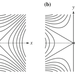
The electric field corresponding to each multipole potential can be obtained by using $\mathbf{E}=-\nabla \Phi$. For example, for the dipolar potential, the corresponding electric field is
$$
\mathbf{E}_{\mathrm{dip}}(\mathbf{x})=-\nabla\left(\frac{\mathbf{p} \cdot \mathbf{x}}{r^{3}}\right)=\frac{\left[3 \mathbf{x}(\mathbf{p} \cdot \mathbf{x})-r^{2} \mathbf{p}\right]}{r^{5}}
$$
电动力学代写
物理代写|电动力学作业代ELECTRODYNAMICS代考|ELECTRIC MULTIPOLE EXPANSION
标量势披(X)由于电荷分布ρ(X′)是(谁)给的
披(X)=∫ρ(X′)|X−X′|d3X′
远离局部电荷分布,观察者将看到总电荷问分布,有效地作为点电荷,并且电位将随着电荷和观察点之间的距离的倒数而下降。然而,即使总费用问为零,标量势在X外电荷分布可能不为零。事实证明披(X)可以用电荷分布几何决定的“多极矩”来表示。我们注意到|X|=r和|X′|=r′. 然后,
1|X−X′|=(X2+X′2−2X⋅X′)−1/2 =1r[1+(r′r)2−2r2∑一世X一世X一世′]−12.
对于电荷分布之外的点,r′≪r, 我们可以使用二项式展开
(1+e)−12=∑n=0∞(−1)n(2n−1)!!n!2nen,
在哪里e=(r′r)2−2r2∑一世X一世X一世′. 所以,
1|X−X′|=1r∑n=0∞(−1)n(2n−1)!!n!2n[(r′r)2−2r2∑一世X一世X一世′] =∑n=0∞(−1)nr2n+1(2n−1)!!n!2n[r′2−2∑一世X一世X一世′]n.
物理代写|电动力学作业代ELECTRODYNAMICS代考|THE ELECTRIC DIPOLE MOMENT
单极矩q是分配的净费用。由于势能中的单极子项下降为1r,它将主导整个潜力r, 每当q非零。电偶极矩p对于任何空间扩展的电荷分布,其中带正电和带负电的成分的“中心”相对于彼此移位,它是非零的。宏观介质中给定的电荷分布具有“永久电偶极矩”,当p在没有电场的情况下是非零的。我们还可以有这样一种情况,即介质中的电偶极矩是由外部电场产生的。这些被称为“诱导偶极矩”。不管电偶极矩的物理起源如何,披d一世p=p⋅Xr3描述远离分布的真正潜力。
通常,多极矩取决于坐标系原点的选择。使用一个简单的示例可以很容易地理解这一点。收取积分q并通过将坐标系的原点从电荷位置移开来计算任何地方的电势。你会看到展开中出现的各种多极势!单极矩q本身是一个标量,因此在坐标变换下是不变的。另一方面,只要净电荷不为零,偶极矩取决于原点的选择。这可以用一个简单的论据来证明。让p′成为原点移动时的“新”偶极矩d这样在“新”坐标系中,X′′=X′+d和ρ(X′′)=ρ(X′). 然后,p′=∫X′′ρ(X′′)d3X′′= ∫(X′+d)ρ(X′)d3X′=p+d∫ρ(X′)d3X′=p+qd. 清楚地,p=p′只有当q=0 .
作为说明,让我们计算两个点电荷的偶极矩±q放置在X′=±12d, 分别。电荷密度可以表示为ρ(X′)= qd(X′−12d)−qd(X′+12d). 使用方程式。3.5, 偶极矩由下式给出
p=∫[qd(X′−12d)−qd(X′+12d)]X′d3X′ =q(12d)−q(−12d)=qd
在这种情况下,净电荷为零,偶极矩p=qd在坐标变换下是不变的。
每个多极电位对应的电场可以通过使用和=−∇披. 例如,对于偶极电位,对应的电场为
和d一世p(X)=−∇(p⋅Xr3)=[3X(p⋅X)−r2p]r5

物理代写|电动力学作业代写electrodynamics代考 请认准UprivateTA™. UprivateTA™为您的留学生涯保驾护航。