如果你也在 怎样代写统计力学statistical mechanics这个学科遇到相关的难题,请随时右上角联系我们的24/7代写客服。统计力学statistical mechanics在物理学中,是一个数学框架,它将统计方法和概率理论应用于大型微观实体的集合。它不假设或假定任何自然法则,而是从这些集合体的行为来解释自然界的宏观行为。
统计力学statistical mechanics产生于经典热力学的发展,对该领域而言,它成功地解释了宏观物理特性–如温度、压力和热容量–以围绕平均值波动的微观参数和概率分布为特征。这建立了统计热力学和统计物理学的领域。
my-assignmentexpert™ 统计力学statistical mechanics作业代写,免费提交作业要求, 满意后付款,成绩80\%以下全额退款,安全省心无顾虑。专业硕 博写手团队,所有订单可靠准时,保证 100% 原创。my-assignmentexpert™, 最高质量的统计力学statistical mechanics作业代写,服务覆盖北美、欧洲、澳洲等 国家。 在代写价格方面,考虑到同学们的经济条件,在保障代写质量的前提下,我们为客户提供最合理的价格。 由于统计Statistics作业种类很多,同时其中的大部分作业在字数上都没有具体要求,因此统计力学statistical mechanics作业代写的价格不固定。通常在经济学专家查看完作业要求之后会给出报价。作业难度和截止日期对价格也有很大的影响。
想知道您作业确定的价格吗? 免费下单以相关学科的专家能了解具体的要求之后在1-3个小时就提出价格。专家的 报价比上列的价格能便宜好几倍。
my-assignmentexpert™ 为您的留学生涯保驾护航 在物理physics作业代写方面已经树立了自己的口碑, 保证靠谱, 高质且原创的物理physics代写服务。我们的专家在统计力学statistical mechanics代写方面经验极为丰富,各种统计力学statistical mechanics相关的作业也就用不着 说。
我们提供的统计力学statistical mechanics及其相关学科的代写,服务范围广, 其中包括但不限于:
- 化学统计力学 chemistry,statistical mechanics
- 非平衡统计力学 Nonequilibrium Statistical Mechanics
- 玻耳兹曼分布律 Boltzmann distribution law
物理代写|统计力学作业代写statistical mechanics代考|Partition function in classical phase space
The aim of this chapter is to formulate without approximation quantum statistical mechanics in classical phase space. To this end expressions for the grand canonical equilibrium partition function and statistical averages are derived. One of the major issues that will recur in later chapters is accounting for the non-commutativity of position and momentum operators in the transformation to classical phase space, a point in which represents the simultaneous specification of the particles’ positions and momenta. A second issue is the accounting for the consequences of wave function symmetrization for bosons and fermions in the continuum of states that is classical phase space.
In section 3.3, it was shown that the symmetrization factor correctly accounted for particle statistics and state occupancy so that a sum over distinct allowed states could be written as a sum over all states with it as weighting factor. At the end of that section, equation (3.29) showed that one did not have to invoke explicitly the symmetrization factor. Instead one could include directly in the sum the symmetrized permutations of the basis functions
$$
\begin{aligned}
\mathrm{TR}^{\prime} \hat{f} &=\frac{1}{N !} \sum_{\mathbf{n}} \chi_{\mathbf{n}}^{\pm}\left\langle\phi_{\mathbf{n}}^{\pm}|\hat{f}| \phi_{\mathbf{n}}^{\pm}\right\rangle \
&=\frac{1}{(N !)^{2}} \sum_{\mathbf{n}} \sum_{\hat{\mathrm{P}}^{\prime}, \hat{\mathrm{P}}^{\prime}}(\pm 1)^{p^{\prime}+p^{\prime \prime}}\left\langle\phi_{\mathbf{n}}\left(\hat{\mathrm{P}}^{\prime} \mathbf{r}\right)|\hat{f}(\mathbf{r})| \phi_{\mathbf{n}}\left(\hat{\mathrm{P}}^{\prime \prime} \mathbf{r}\right)\right\rangle \
&=\frac{1}{N !} \sum_{\mathbf{n}} \sum_{\hat{\mathrm{p}}}(\pm 1)^{p}\left\langle\phi_{\mathbf{n}}\left(\hat{\mathrm{P}} \mathbf{r}^{\prime \prime}\right)\left|\hat{f}\left(\mathbf{r}^{\prime \prime}\right)\right| \phi_{\mathbf{n}}\left(\mathbf{r}^{\prime \prime}\right)\right\rangle .
\end{aligned}
$$
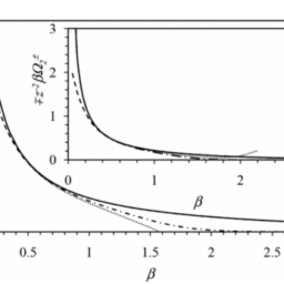
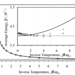
物理代写|统计力学作业代写statistical mechanics代考|Loop expansion, grand potential and average energy
As discussed in section 3.4.2, any particular particle permutation operator can be factored into loop permutation operators, where a loop is a closed connected sequence of successive pair transpositions. Hence the sum over all permutation operators can be written as the sum over all possible factors of loop permutations, equation (3.44)
$$
\sum_{\hat{\mathrm{P}}}(\pm 1)^{p} \hat{\mathrm{P}}=\hat{\mathrm{I}} \pm \sum_{i, j}^{\prime} \hat{\mathrm{P}}{i j}+\sum{i, j, k}^{\prime} \hat{\mathrm{P}}{i j} \hat{\mathrm{P}}{j k}+\sum_{i, j, k, l}^{\prime} \hat{\mathrm{P}}{i j} \hat{\mathrm{P}}{k l} \pm \ldots
$$
Here $\hat{\mathrm{P}}_{j k}$ is the transpose of particles $j$ and $k$. The prime on the sums restrict them to unique loops, with each index being different. The first term is just the identity. The second term is a dimer loop, the third term is a trimer loop, and the fourth term shown is the product of two different dimers.
With this, the symmetrization function, $\eta_{\mathrm{q}}^{\pm}(\boldsymbol{\Gamma})=\sum_{\hat{\mathbf{P}}}(\pm 1)^{p}\langle\hat{\mathrm{P}} \mathbf{p} \mid \mathbf{q}\rangle /\langle\mathbf{p} \mid \mathbf{q}\rangle$, is the sum of the expectation values of these loops. The monomer symmetrization function is obviously unity, $\eta_{\mathrm{q}}^{(1)} \equiv\langle\mathbf{p} \mid \mathbf{q}\rangle /\langle\mathbf{p} \mid \mathbf{q}\rangle=1$.
The dimer symmetrization function in the microstate $\boldsymbol{\Gamma}$ for particles $j$ and $k$ is
$$
\begin{aligned}
\eta_{\mathbf{q} ; j k}^{\pm(2)} &=\frac{\pm\left\langle\hat{\mathbf{P}}{j k} \mathbf{p} \mid \mathbf{q}\right\rangle}{\langle\mathbf{p} \mid \mathbf{q}\rangle} \ &=\frac{\pm\left\langle\mathbf{p}{k} \mid \mathbf{q}{j}\right\rangle\left\langle\mathbf{p}{j} \mid \mathbf{q}{k}\right\rangle}{\left\langle\mathbf{p}{j} \mid \mathbf{q}{j}\right\rangle\left\langle\mathbf{p}{k} \mid \mathbf{q}{k}\right\rangle} \ &=\pm e^{\left(\mathbf{q}{k}-\mathbf{q}{j}\right) \cdot \mathbf{p} j / i \hbar} e^{\left(\mathbf{q}{j}-\mathbf{q}{k}\right) \cdot \mathbf{p}{k} / i \hbar}
\end{aligned}
$$ single-particle functions, the expectation value factorizes leaving only the permuted particles to contribute (cf section 3.4.3).
Similarly the trimer symmetrization function for particles $j, k$, and $l$ is
$$
\begin{aligned}
\eta_{\mathrm{q} ; j k l}^{\pm(3)} &=\frac{\left\langle\hat{\mathrm{P}}{j k} \hat{\mathbf{P}}{k l} \mathbf{p} \mid \mathbf{q}\right\rangle}{\langle\mathbf{p} \mid \mathbf{q}\rangle} \
&=\frac{\left\langle\mathbf{p}{k} \mid \mathbf{q}{j}\right\rangle\left\langle\mathbf{p}{j} \mid \mathbf{q}{l}\right\rangle\left\langle\mathbf{p}{l} \mid \mathbf{q}{k}\right\rangle}{\left\langle\mathbf{p}{j} \mid \mathbf{q}{j}\right\rangle\left\langle\mathbf{p}{k} \mid \mathbf{q}{k}\right\rangle\left\langle\mathbf{p}{l} \mid \mathbf{q}{l}\right\rangle} \
&=e^{\left(\mathbf{q}{j}-\mathbf{q}{k}\right) \cdot \mathbf{p}{k} / i h^{\prime} e^{\left(\mathbf{q}{k}-\mathbf{q}{l} / \mathbf{p}{l} / i h^{\prime}\right.} e^{\left(\mathbf{q}{l}-\mathbf{q}{j}\right) \cdot \mathbf{p} / / i h}} .
\end{aligned}
$$
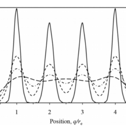
物理代写|统计力学作业代写STATISTICAL MECHANICS代考|Multi-particle density
Consider a position configuration of $n$ particles, $\mathbf{Q}^{n}=\left{\mathbf{Q}{1}, \mathbf{Q}{2}, \ldots, \mathbf{Q}{n}\right}$. The distinct $n$-particle density quantum operator for this is $$ \hat{\rho}^{(n)}\left(\mathbf{Q}^{n} ; \mathbf{r}\right)=\sum{k_{1}, \ldots, k_{n}}^{N} \prod_{j=1}^{n} \delta\left(\mathbf{Q}{j}-\mathbf{r}{k_{j}}\right) .
$$
The sum is over the particle indeces, and the double prime indicates that in any term no two indeces are equal. If there are $N$ particles in the system, then there are $N ! /(N-n) !$ terms in the sum. This says any particle is at $\mathbf{Q}{1}$, any different particle is at $\mathbf{Q}{2}$, etc. The density operator is evidently unchanged by a permutation of the $\mathbf{Q}_{j}$ or of the particle labels.
Since this is only a function of the position operator, the commutation function $\omega_{\mathrm{q}}$ or $\omega_{\mathrm{p}}$ may be used for its average. The average $n$-particle density is
$$
\begin{aligned}
\rho_{\omega_{p} \eta_{q}^{\pm}}^{(n)} &\left(\mathbf{Q}^{n}\right) \
& \equiv\left\langle\hat{\rho}^{(n)}\left(\mathbf{Q}^{n} ; \mathbf{q}\right)\right\rangle_{\omega_{p} \eta_{q}^{\pm}} \
&=\frac{1}{\Xi_{\omega_{p} \eta_{q}^{\pm}}} \sum_{N=0}^{\infty} \frac{z^{N}}{h^{d N} N !} \int \mathrm{d} \boldsymbol{\Gamma} e^{-\beta \mathcal{H}(\mathbf{\Gamma})} \omega_{\mathrm{p}}(\boldsymbol{\Gamma}) \eta_{\mathrm{q}}^{\pm}(\boldsymbol{\Gamma}) \sum_{k_{\mathrm{b}}, \ldots, k_{n}}^{N} \prod_{j=1}^{n} \delta\left(\mathbf{Q}{j}-\mathbf{q}{k_{j}}\right) .
\end{aligned}
$$
It is worth mentioning that one does not actually have to define the quantum operator density, $\hat{\rho}^{(n)}\left(\mathbf{Q}^{n} ; \mathbf{q}\right)$, but that instead one can introduce the phase function $\rho_{\omega_{\mathrm{p}}}^{(n)}\left(\mathbf{Q}^{n}\right)$ directly via the phase space integral. More generally one can define the $n$ particle density for positions and momenta in phase space as
$$
\rho^{(n)}\left(\gamma^{n} ; \mathbf{\Gamma}\right)=\sum_{k_{1}, \ldots, k_{n}}^{N} \prod_{j=1}^{n} \delta\left(\gamma_{j}-\boldsymbol{\Gamma}{k{j}}\right),
$$
and its average as
$$
\begin{aligned}
\rho_{\omega_{p} \eta_{q}^{\pm}}^{(n)}\left(\gamma^{n}\right) \equiv & \frac{1}{\Xi_{\omega_{p} \eta_{q}^{\pm}}} \sum_{N=0}^{\infty} \frac{z^{N}}{h^{d N} N !} \int \mathrm{d} \boldsymbol{\Gamma} e^{-\beta \mathcal{H}(\mathbf{\Gamma})} \omega_{\mathrm{p}}(\mathbf{\Gamma}) \eta_{\mathrm{q}}^{\pm}(\mathbf{\Gamma}) \
& \times \sum_{k_{1}, \ldots, k_{n}}^{N} \prod_{j=1}^{n} \delta\left(\gamma_{j}-\boldsymbol{\Gamma}{k{j}}\right) .
\end{aligned}
$$
统计力学代考
物理代写|统计力学作业代写STATISTICAL MECHANICS代考|PARTITION FUNCTION IN CLASSICAL PHASE SPACE
本章的目的是在经典相空间中建立不带近似的量子统计力学。为此,导出了大规范平衡分配函数和统计平均值的表达式。在后面的章节中将重复出现的主要问题之一是解释位置和动量算子在转换到经典相空间中的非交换性,这一点表示粒子位置和动量的同时指定。第二个问题是解释波函数对称化对经典相空间状态连续体中玻色子和费米子的影响。
在第 3.3 节中,证明了对称因子正确地解释了粒子统计和状态占有率,因此不同允许状态的总和可以写成所有状态的总和,并将其作为加权因子。在该部分的末尾,等式3.29表明不必明确调用对称因子。相反,可以将基函数的对称排列直接包含在总和中
吨R′F^=1ñ!∑nχn±⟨φn±|F^|φn±⟩ =1(ñ!)2∑n∑磷^′,磷^′(±1)p′+p′′⟨φn(磷^′r)|F^(r)|φn(磷^′′r)⟩ =1ñ!∑n∑p^(±1)p⟨φn(磷^r′′)|F^(r′′)|φn(r′′)⟩.
物理代写|统计力学作业代写STATISTICAL MECHANICS代考|LOOP EXPANSION, GRAND POTENTIAL AND AVERAGE ENERGY
如第 3.4.2 节所述,任何特定的粒子置换算子都可以分解为循环置换算子,其中循环是连续对转置的闭合连接序列。因此,所有置换算子的总和可以写成循环置换的所有可能因子的总和,等式3.44
$$
\sum_{\hat{\mathrm{P}}}(\pm 1)^{p} \hat{\mathrm{P}}=\hat{\mathrm{I}} \pm \sum_{i, j}^{\prime} \hat{\mathrm{P}}{i j}+\sum{i, j, k}^{\prime} \hat{\mathrm{P}}{i j} \hat{\mathrm{P}}{j k}+\sum_{i, j, k, l}^{\prime} \hat{\mathrm{P}}{i j} \hat{\mathrm{P}}{k l} \pm \ldots
$$
这里磷^jķ是粒子的转置j和ķ. 总和上的素数将它们限制为唯一的循环,每个索引都不同。第一项只是身份。第二项是二聚体环,第三项是三聚体环,显示的第四项是两个不同二聚体的产物。
有了这个,对称化函数,这q±(Γ)=∑磷^(±1)p⟨磷^p∣q⟩/⟨p∣q⟩, 是这些循环的期望值的总和。单体对称化函数明显统一,这q(1)≡⟨p∣q⟩/⟨p∣q⟩=1.
微观状态下的二聚体对称函数Γ用于粒子j和ķ是
$\boldsymbol{\Gamma}$ for particles $j$ and $k$ is
$$
\begin{aligned}
\eta_{\mathbf{q} ; j k}^{\pm(2)} &=\frac{\pm\left\langle\hat{\mathbf{P}}{j k} \mathbf{p} \mid \mathbf{q}\right\rangle}{\langle\mathbf{p} \mid \mathbf{q}\rangle} \ &=\frac{\pm\left\langle\mathbf{p}{k} \mid \mathbf{q}{j}\right\rangle\left\langle\mathbf{p}{j} \mid \mathbf{q}{k}\right\rangle}{\left\langle\mathbf{p}{j} \mid \mathbf{q}{j}\right\rangle\left\langle\mathbf{p}{k} \mid \mathbf{q}{k}\right\rangle} \ &=\pm e^{\left(\mathbf{q}{k}-\mathbf{q}{j}\right) \cdot \mathbf{p} j / i \hbar} e^{\left(\mathbf{q}{j}-\mathbf{q}{k}\right) \cdot \mathbf{p}{k} / i \hbar}
\end{aligned}
$$ single-particle functions, the expectation value factorizes leaving only the permuted particles to contribute (cf section 3.4.3).
Similarly the trimer symmetrization function for particles $j, k$, and $l$ is
$$
\begin{aligned}
\eta_{\mathrm{q} ; j k l}^{\pm(3)} &=\frac{\left\langle\hat{\mathrm{P}}{j k} \hat{\mathbf{P}}{k l} \mathbf{p} \mid \mathbf{q}\right\rangle}{\langle\mathbf{p} \mid \mathbf{q}\rangle} \
&=\frac{\left\langle\mathbf{p}{k} \mid \mathbf{q}{j}\right\rangle\left\langle\mathbf{p}{j} \mid \mathbf{q}{l}\right\rangle\left\langle\mathbf{p}{l} \mid \mathbf{q}{k}\right\rangle}{\left\langle\mathbf{p}{j} \mid \mathbf{q}{j}\right\rangle\left\langle\mathbf{p}{k} \mid \mathbf{q}{k}\right\rangle\left\langle\mathbf{p}{l} \mid \mathbf{q}{l}\right\rangle} \
&=e^{\left(\mathbf{q}{j}-\mathbf{q}{k}\right) \cdot \mathbf{p}{k} / i h^{\prime} e^{\left(\mathbf{q}{k}-\mathbf{q}{l} / \mathbf{p}{l} / i h^{\prime}\right.} e^{\left(\mathbf{q}{l}-\mathbf{q}{j}\right) \cdot \mathbf{p} / / i h}} .
\end{aligned}
$$
物理代写|统计力学作业代写STATISTICAL MECHANICS代考|MULTI-PARTICLE DENSITY
考虑一个位置配置n粒子, $\mathbf{Q}^{n}=\left{\mathbf{Q}{1}, \mathbf{Q}{2}, \ldots, \mathbf{Q}{n}\right}$. The distinct $n$-particle density quantum operator for this is $$ \hat{\rho}^{(n)}\left(\mathbf{Q}^{n} ; \mathbf{r}\right)=\sum{k_{1}, \ldots, k_{n}}^{N} \prod_{j=1}^{n} \delta\left(\mathbf{Q}{j}-\mathbf{r}{k_{j}}\right) .
$$
总和超过了粒子索引,双素数表示在任何项中没有两个索引是相等的。如果有ñ系统中的粒子,则有ñ!/(ñ−n)!总和中的条款。这表示任何粒子都在 $\mathbf{Q} {1},一种n是d一世FF和r和n吨p一种r吨一世Cl和一世s一种吨\mathbf{Q} {2},和吨C.吨H和d和ns一世吨是这p和r一种吨这r一世s和在一世d和n吨l是在nCH一种nG和db是一种p和r米在吨一种吨一世这n这F吨H和\mathbf{Q}_{j}$ 或粒子标签。
因为这只是位置算子的一个函数,所以换向函数ωq或者ωp可用于其平均值。平均值n-粒子密度为
$$\omega_{\mathrm{q}}$ or $\omega_{\mathrm{p}}$ may be used for its average. The average $n$-particle density is
$$
\begin{aligned}
\rho_{\omega_{p} \eta_{q}^{\pm}}^{(n)} &\left(\mathbf{Q}^{n}\right) \
& \equiv\left\langle\hat{\rho}^{(n)}\left(\mathbf{Q}^{n} ; \mathbf{q}\right)\right\rangle_{\omega_{p} \eta_{q}^{\pm}} \
&=\frac{1}{\Xi_{\omega_{p} \eta_{q}^{\pm}}} \sum_{N=0}^{\infty} \frac{z^{N}}{h^{d N} N !} \int \mathrm{d} \boldsymbol{\Gamma} e^{-\beta \mathcal{H}(\mathbf{\Gamma})} \omega_{\mathrm{p}}(\boldsymbol{\Gamma}) \eta_{\mathrm{q}}^{\pm}(\boldsymbol{\Gamma}) \sum_{k_{\mathrm{b}}, \ldots, k_{n}}^{N} \prod_{j=1}^{n} \delta\left(\mathbf{Q}{j}-\mathbf{q}{k_{j}}\right) .
\end{aligned}
$$
It is worth mentioning that one does not actually have to define the quantum operator density, $\hat{\rho}^{(n)}\left(\mathbf{Q}^{n} ; \mathbf{q}\right)$, but that instead one can introduce the phase function $\rho_{\omega_{\mathrm{p}}}^{(n)}\left(\mathbf{Q}^{n}\right)$ directly via the phase space integral. More generally one can define the $n$ particle density for positions and momenta in phase space as
$$
\rho^{(n)}\left(\gamma^{n} ; \mathbf{\Gamma}\right)=\sum_{k_{1}, \ldots, k_{n}}^{N} \prod_{j=1}^{n} \delta\left(\gamma_{j}-\boldsymbol{\Gamma}{k{j}}\right),
$$
and its average as
$$
\begin{aligned}
\rho_{\omega_{p} \eta_{q}^{\pm}}^{(n)}\left(\gamma^{n}\right) \equiv & \frac{1}{\Xi_{\omega_{p} \eta_{q}^{\pm}}} \sum_{N=0}^{\infty} \frac{z^{N}}{h^{d N} N !} \int \mathrm{d} \boldsymbol{\Gamma} e^{-\beta \mathcal{H}(\mathbf{\Gamma})} \omega_{\mathrm{p}}(\mathbf{\Gamma}) \eta_{\mathrm{q}}^{\pm}(\mathbf{\Gamma}) \
& \times \sum_{k_{1}, \ldots, k_{n}}^{N} \prod_{j=1}^{n} \delta\left(\gamma_{j}-\boldsymbol{\Gamma}{k{j}}\right) .
\end{aligned}
$$

物理代写|统计力学作业代写statistical mechanics代考 请认准UprivateTA™. UprivateTA™为您的留学生涯保驾护航。
电磁学代考
物理代考服务:
物理Physics考试代考、留学生物理online exam代考、电磁学代考、热力学代考、相对论代考、电动力学代考、电磁学代考、分析力学代考、澳洲物理代考、北美物理考试代考、美国留学生物理final exam代考、加拿大物理midterm代考、澳洲物理online exam代考、英国物理online quiz代考等。
光学代考
光学(Optics),是物理学的分支,主要是研究光的现象、性质与应用,包括光与物质之间的相互作用、光学仪器的制作。光学通常研究红外线、紫外线及可见光的物理行为。因为光是电磁波,其它形式的电磁辐射,例如X射线、微波、电磁辐射及无线电波等等也具有类似光的特性。
大多数常见的光学现象都可以用经典电动力学理论来说明。但是,通常这全套理论很难实际应用,必需先假定简单模型。几何光学的模型最为容易使用。
相对论代考
上至高压线,下至发电机,只要用到电的地方就有相对论效应存在!相对论是关于时空和引力的理论,主要由爱因斯坦创立,相对论的提出给物理学带来了革命性的变化,被誉为现代物理性最伟大的基础理论。
流体力学代考
流体力学是力学的一个分支。 主要研究在各种力的作用下流体本身的状态,以及流体和固体壁面、流体和流体之间、流体与其他运动形态之间的相互作用的力学分支。
随机过程代写
随机过程,是依赖于参数的一组随机变量的全体,参数通常是时间。 随机变量是随机现象的数量表现,其取值随着偶然因素的影响而改变。 例如,某商店在从时间t0到时间tK这段时间内接待顾客的人数,就是依赖于时间t的一组随机变量,即随机过程
Matlab代写
MATLAB 是一种用于技术计算的高性能语言。它将计算、可视化和编程集成在一个易于使用的环境中,其中问题和解决方案以熟悉的数学符号表示。典型用途包括:数学和计算算法开发建模、仿真和原型制作数据分析、探索和可视化科学和工程图形应用程序开发,包括图形用户界面构建MATLAB 是一个交互式系统,其基本数据元素是一个不需要维度的数组。这使您可以解决许多技术计算问题,尤其是那些具有矩阵和向量公式的问题,而只需用 C 或 Fortran 等标量非交互式语言编写程序所需的时间的一小部分。MATLAB 名称代表矩阵实验室。MATLAB 最初的编写目的是提供对由 LINPACK 和 EISPACK 项目开发的矩阵软件的轻松访问,这两个项目共同代表了矩阵计算软件的最新技术。MATLAB 经过多年的发展,得到了许多用户的投入。在大学环境中,它是数学、工程和科学入门和高级课程的标准教学工具。在工业领域,MATLAB 是高效研究、开发和分析的首选工具。MATLAB 具有一系列称为工具箱的特定于应用程序的解决方案。对于大多数 MATLAB 用户来说非常重要,工具箱允许您学习和应用专业技术。工具箱是 MATLAB 函数(M 文件)的综合集合,可扩展 MATLAB 环境以解决特定类别的问题。可用工具箱的领域包括信号处理、控制系统、神经网络、模糊逻辑、小波、仿真等。