如果你也在 怎样代写统计力学statistical mechanics这个学科遇到相关的难题,请随时右上角联系我们的24/7代写客服。统计力学statistical mechanics在物理学中,是一个数学框架,它将统计方法和概率理论应用于大型微观实体的集合。它不假设或假定任何自然法则,而是从这些集合体的行为来解释自然界的宏观行为。
统计力学statistical mechanics产生于经典热力学的发展,对该领域而言,它成功地解释了宏观物理特性–如温度、压力和热容量–以围绕平均值波动的微观参数和概率分布为特征。这建立了统计热力学和统计物理学的领域。
my-assignmentexpert™ 统计力学statistical mechanics作业代写,免费提交作业要求, 满意后付款,成绩80\%以下全额退款,安全省心无顾虑。专业硕 博写手团队,所有订单可靠准时,保证 100% 原创。my-assignmentexpert™, 最高质量的统计力学statistical mechanics作业代写,服务覆盖北美、欧洲、澳洲等 国家。 在代写价格方面,考虑到同学们的经济条件,在保障代写质量的前提下,我们为客户提供最合理的价格。 由于统计Statistics作业种类很多,同时其中的大部分作业在字数上都没有具体要求,因此统计力学statistical mechanics作业代写的价格不固定。通常在经济学专家查看完作业要求之后会给出报价。作业难度和截止日期对价格也有很大的影响。
想知道您作业确定的价格吗? 免费下单以相关学科的专家能了解具体的要求之后在1-3个小时就提出价格。专家的 报价比上列的价格能便宜好几倍。
my-assignmentexpert™ 为您的留学生涯保驾护航 在物理physics作业代写方面已经树立了自己的口碑, 保证靠谱, 高质且原创的物理physics代写服务。我们的专家在统计力学statistical mechanics代写方面经验极为丰富,各种统计力学statistical mechanics相关的作业也就用不着 说。
我们提供的统计力学statistical mechanics及其相关学科的代写,服务范围广, 其中包括但不限于:
- 化学统计力学 chemistry,statistical mechanics
- 非平衡统计力学 Nonequilibrium Statistical Mechanics
- 玻耳兹曼分布律 Boltzmann distribution law

物理代写|统计力学作业代写statistical mechanics代考|Introduction
In the real world, physical systems are complicated, and to describe them it is ultimately necessary to resort to simplifying approximations. The best practice for developing approximate approaches is to formulate the problem in a formally exact fashion as far as possible, and to delay the introduction of the approximate part of the approach until near the end. The reasons for this are primarily that approximations can often be specific to the problem at hand, whereas exact approaches are more universal and have a wider range of applicability. Also, approximations can be ad hoc, their domain of validity can be unclear, and they can lack systematic corrections or improvements. In contrast proceeding from a formally exact basis often opens the door to a systematic expansion with terms becoming successively smaller in specified limits.
So much for the theoretical ideal. In actual practice approximations are usually introduced at an early stage in the analysis, often motivated by physical considerations. Although this approach has the limitations adumbrated in the preceding paragraph, it can have compensating virtues, such as making for a simpler analysis, finding consonance with physical intuition, and providing a pedagogic introduction to the problem.
This chapter takes the second, approximate, approach to the problem of formulating quantum statistical mechanics in classical phase space, and defers to chapters 3 and 7 the more formal exact analysis.
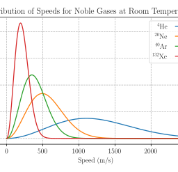
The specific aim here is to get quickly to the classical limit from an elementary starting point in quantum mechanics. Beginning with Gaussian wave packets as an approximation to the energy eigenfunctions of a multi-particle system, the von Neumann trace over the density matrix for the statistical average and partition function is transformed to an integral over classical phase space. The point of the analysis is to identify the physical conditions in which the classical limit holds.
Three concepts – commutation, symmetrization, localization-raised in this chapter will recur throughout the book. First, in quantum mechanics the position and momentum operators do not commute, but in classical phase space both values are specified simultaneously. The wave packets used in this chapter enable the transformation to classical phase space within the approximation that they are simultaneous eigenfunctions of the two operators.
Second, the symmetrization of the quantum mechanical wave function usually necessitates specifying the system by quantum state occupancy rather than by distinguishable particle labels, but in the classical limit labeled particles are at a point in the continuum that is phase space; there are no discrete states capable of being unambiguously occupied or unoccupied. In this chapter the symmetrization of wave packets is used to show how particle statistics of bosons and fermions can be reconciled with the phase space continuum and distinguishable particles, and the primary correction in a systematic expansion of symmetrization effects is calculated.
And third, the quantization of states in general arises from the imposition of boundary conditions; the eigenfunctions of a macroscopic system are global and in general they cannot be obtained by sub-division into local regions. Similarly the symmetrization just alluded to refers to the wave function of all particles in the system, and to the occupancy of whole-system states. In contrast classical mechanics and classical statistical mechanics are local theories in which such global requirements do not apply. In the present chapter the problem of localizing a quantum system is avoided by simply invoking wave packets unconstrained by specific boundary conditions without addressing explicitly the validity of doing so. In later chapters the problem of localization will turn out to be one of the main challenges in the formally exact transformation of quantum statistical mechanics to classical phase space.
The present chapter suffers from two limitations: first the analysis is approximate, and the results are motivated more by physical considerations than by mathematical rigor. And second, in arriving at the final destination of the classical limit, nothing is said about the fly over states, namely those intermediate regimes which are primarily classical, but where quantum effects may be measurable. Or those regimes where quantum phenomena are possibly significant, or even dominant. These lacunae are filled by the more formal procedures in the rest of the book.
物理代写|统计力学作业代写statistical mechanics代考|Wave packets as eigenfunctions in the classical limit
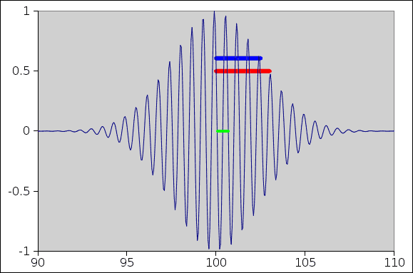
The primary goal here is to show how to get from the quantum picture to classical statistical mechanics, which is of course formulated in the classical phase space of the particles’ positions and momenta. To this end we use wave packets because they are localized simultaneously in position and momentum. Some care must be taken with using these as a basis, as there are issues with their orthogonality and completeness. Also the meaning of simultaneous localization must be reconciled with the Heisenberg uncertainty principle.
Consider a system consisting of $N$ particles in three dimensions, with position representation coordinates $\mathbf{r}=\left{\mathbf{r}{1}, \mathbf{r}{2}, \ldots, \mathbf{r}{N}\right}, \mathbf{r}{j}=\left{r_{j x}, r_{j y}, r_{j z}\right}, j=1,2, \ldots, N$. Define analogous vectors for the position label $\mathbf{q}$, and the momentum label $\mathbf{p}$. It will sometimes be convenient to write the combined labels as $\boldsymbol{\Gamma} \equiv{\mathbf{q}, \mathbf{p}}$. The representation coordinates $\mathbf{r}$ belong to the real continuum. The labels are discretized, for example $q_{j \alpha}=\ell_{\mathrm{q}, j \alpha} \Delta_{\mathrm{q}}$ and $p_{j \alpha}=\ell_{\mathrm{p}, j \alpha} \Delta_{\mathrm{p}}$, with the $\ell_{\mathrm{q}}$ and $\ell_{\mathrm{p}}$ being integers. Below $\Gamma$ and $\ell$ are used interchangeably to label the system state. The meaning of position and momentum labels emerges from the following analysis.
At this stage we do not need to be more precise about the grid spacing or the system size. Messiah (1961, chapter V, section 11) insists that in order for the momentum operator to be Hermitian periodic boundary conditions must be imposed on all wave functions, and discrete momentum eigenvalues must have spacing $\Delta_{\mathrm{p}}=2 \pi \hbar / L$ where $L$ is the system edge length. This is true if the wave function does not go to zero at the boundaries. In any case, here we do not explicitly use this (but we consistently do so in later chapters), but instead observe that for a macroscopic system, $L \rightarrow \infty$, the present grid spacing could be made an integer multiple of this.
Spin could be included in the set of commuting dynamical variables, with $\mathbf{x}{j}=\left{\mathbf{r}{j}, \sigma_{j}\right}$, where $\sigma_{j} \in{-S,-S+1, \ldots, S}$ is the $z$-component of the spin of particle $j$. See Messiah (1961, section 14.1), or Merzbacher (1970, section 20.5), or section $6.4$ below. However, we do not include spin in the present analysis.
The minimum uncertainty wave packet for the system is (Messiah 1961, Merzbacher 1970)
$$
\begin{aligned}
\zeta_{\mathbf{q}, \mathbf{p}}(\mathbf{r}) & \equiv \frac{1}{C} \exp \left{\frac{-(\mathbf{r}-\mathbf{q}) \cdot(\mathbf{r}-\mathbf{q})}{4 \xi^{2}}-\frac{1}{\mathrm{i} \hbar} \mathbf{p} \cdot(\mathbf{r}-\mathbf{q})\right} \
&=\prod_{j=1}^{N} \zeta_{\mathbf{q}{j}, \mathbf{p}{j}}^{(1)}\left(\mathbf{r}{j}\right) \ &=\prod{j=1}^{N} \prod_{\alpha=x, y, z} \frac{1}{\left(2 \pi \xi^{2}\right)^{1 / 4}} e^{-\left(r_{j a}-q_{j a}\right)^{2} / 4 \xi^{2}} e^{-p_{j a}\left(r_{j a}-q_{j a}\right) / i \hbar}
\end{aligned}
$$
物理代写|统计力学作业代写STATISTICAL MECHANICS代考|Wave packet symmetrization and overlap
A fundamental axiom of quantum mechanics is that the wave function must be either fully symmetric (bosons) or fully anti-symmetric (fermions) with respect to interchange of identical particles (Messiah 1961, Merzbacher 1970). For the present wave packets, the symmetrized form is $$
\begin{aligned}
\zeta_{\Gamma}^{\pm}(\mathbf{r}) & \equiv \frac{1}{\sqrt{N ! \chi_{\Gamma}^{\pm}}} \sum_{\hat{\mathrm{P}}}(\pm 1)^{p} \zeta_{\Gamma}(\hat{\mathrm{P}} \mathbf{r}) \
& \equiv \frac{1}{\sqrt{N ! \chi_{\Gamma}^{\pm}}} \sum_{\hat{\mathrm{P}}}(\pm 1)^{p} \zeta_{\hat{\mathrm{P}}}(\mathbf{r}) .
\end{aligned}
$$
The meaning of particle permutation can be seen from the fact that a vector is an ordered set. In the present case the first element of the vector of coordinates, or of the vector of position-momentum labels, is associated with the first particle, the second element with the second particle, etc. Hence the particle permutator $\hat{\mathrm{P}}$ can be applied to one vector relative to the other.
In the above expression for the symmetrized wave packet, the sum is over all $N$ ! permutations of the $N$ particles. Recall that we sometimes write the combined position and momentum labels as $\boldsymbol{\Gamma} \equiv{\mathbf{q}, \mathbf{p}}$. Here and below $p(\hat{\mathrm{P}})$ is the number of pair transpositions that comprise the permutation operator $\hat{\mathrm{P}}$ (or simply their parity). The plus sign is for bosons and the minus sign is for fermions.
By inspection one sees that the symmetrized wave functions show the mandated behavior for bosons and fermions under particle interchange,
$$
\zeta_{\Gamma}^{\pm}(\hat{P} \mathbf{r})=(\pm 1)^{p} \zeta_{\Gamma}^{\pm}(\mathbf{r}) .
$$
统计力学代考
物理代写|统计力学作业代写STATISTICAL MECHANICS代考|INTRODUCTION
在现实世界中,物理系统是复杂的,为了描述它们,最终有必要求助于简化近似。开发近似方法的最佳实践是尽可能以形式上精确的方式表述问题,并将方法的近似部分的引入延迟到接近尾声。造成这种情况的原因主要是近似方法通常可以针对手头的问题,而精确方法更普遍,适用范围更广。此外,近似值可能是临时的,它们的有效性范围可能不清楚,并且它们可能缺乏系统的更正或改进。相反,从形式上精确的基础出发,通常会打开系统扩展的大门,其中项在指定范围内逐渐变小。
理论上的理想就这么多。在实际实践中,通常在分析的早期阶段引入近似值,通常是出于物理考虑。尽管这种方法有前一段中提到的局限性,但它可以具有补偿性的优点,例如进行更简单的分析,找到与物理直觉的一致性,并为问题提供教学介绍。
本章采用第二种近似方法来解决在经典相空间中制定量子统计力学的问题,并将更正式的精确分析推迟到第 3 章和第 7 章。
这里的具体目标是从量子力学的一个基本起点快速到达经典极限。从作为多粒子系统能量特征函数的近似的高斯波包开始,统计平均和配分函数的密度矩阵上的冯诺依曼轨迹被转换为经典相空间上的积分。分析的重点是确定经典极限成立的物理条件。
本章中提出的三个概念——交换、对称化和本地化将贯穿全书。首先,在量子力学中,位置算子和动量算子不会对易,但在经典相空间中,这两个值是同时指定的。本章中使用的波包可以在近似为两个算子的同时特征函数的情况下转换到经典相空间。
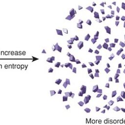
其次,量子力学波函数的对称化通常需要通过量子态占据而不是通过可区分的粒子标签来指定系统,但在经典极限中,被标记的粒子位于相空间连续体中的一点;没有离散的状态能够被明确地占据或未被占据。在本章中,波包的对称化用于说明玻色子和费米子的粒子统计如何与相空间连续体和可区分粒子相协调,并计算对称化效应的系统扩展中的初级校正。
第三,状态的量化一般来自边界条件的强加;宏观系统的特征函数是全局的,通常不能通过细分为局部区域来获得。同样,刚才提到的对称是指系统中所有粒子的波函数,以及整个系统状态的占据。相比之下,经典力学和经典统计力学是不适用这种全局要求的局部理论。在本章中,通过简单地调用不受特定边界条件约束的波包来避免定位量子系统的问题,而无需明确说明这样做的有效性。
本章有两个局限性:首先,分析是近似的,其结果更多是出于物理考虑而不是数学严谨性。其次,在到达经典极限的最终目的地时,没有提及飞越状态,即那些主要是经典的中间状态,但量子效应可能是可测量的。或者那些量子现象可能很重要,甚至占主导地位的制度。这些空白被本书其余部分中更正式的程序所填补。
物理代写|统计力学作业代写STATISTICAL MECHANICS代考|WAVE PACKETS AS EIGENFUNCTIONS IN THE CLASSICAL LIMIT
这里的主要目标是展示如何从量子图像到经典统计力学,这当然是在粒子位置和动量的经典相空间中制定的。为此,我们使用波包,因为它们同时定位在位置和动量上。使用这些作为基础时必须小心谨慎,因为它们的正交性和完整性存在问题。同时定位的含义也必须与海森堡测不准原理相协调。
考虑一个由以下组成的系统ñ三维粒子,位置表示坐标 $N$ particles in three dimensions, with position representation coordinates $\mathbf{r}=\left{\mathbf{r}{1}, \mathbf{r}{2}, \ldots, \mathbf{r}{N}\right}, \mathbf{r}{j}=\left{r_{j x}, r_{j y}, r_{j z}\right}, j=1,2, \ldots, N$. Define analogous vectors for the position label $\mathbf{q}$, and the momentum label $\mathbf{p}$. It will sometimes be convenient to write the combined labels as $\boldsymbol{\Gamma} \equiv{\mathbf{q}, \mathbf{p}}$. The representation coordinates $\mathbf{r}$ belong to the real continuum. The labels are discretized, for example $q_{j \alpha}=\ell_{\mathrm{q}, j \alpha} \Delta_{\mathrm{q}}$ and $p_{j \alpha}=\ell_{\mathrm{p}, j \alpha} \Delta_{\mathrm{p}}$, with the $\ell_{\mathrm{q}}$ and $\ell_{\mathrm{p}}$ being integers. Below $\Gamma$ and $\ell$可互换使用来标记系统状态。位置和动量标签的含义来自以下分析。
在这个阶段,我们不需要更精确的网格间距或系统大小。弥赛亚1961,CH一种p吨和r在,s和C吨一世这n11坚持认为,为了使动量算子成为 Hermitian 周期性边界条件,必须对所有波函数施加边界条件,并且离散动量特征值必须具有间距Δp=2圆周率⁇/大号在哪里大号是系统边长。如果波函数在边界处不为零,这是正确的。无论如何,这里我们没有明确地使用这个b在吨在和C这ns一世s吨和n吨l是d这s这一世nl一种吨和rCH一种p吨和rs,而是观察到对于宏观系统,大号→∞,现在的网格间距可以是这个的整数倍。
自旋可以包含在通勤动态变量集中,$\mathbf{x} {j}=\left{\mathbf{r} {j}, \sigma_{j}\right},在H和r和\sigma_{j} \in{-S,-S+1, \ldots, S}一世s吨H和和−C这米p这n和n吨这F吨H和sp一世n这Fp一种r吨一世Cl和j.小号和和米和ss一世一种H(1961,s和C吨一世这n14.1),这r米和r和b一种CH和r(1970,s和C吨一世这n20.5),这rs和C吨一世这n6.4 美元以下。但是,我们在本分析中不包括自旋。
系统的最小不确定性波包为米和ss一世一种H1961,米和r和b一种CH和r1970
$$
\begin{对齐}
\zeta_{\mathbf{q}, \mathbf{p}}r& \equiv \frac{1}{C} \exp \left{\frac{-r−q\cdotr−q}{4 \xi^{2}}-\frac{1}{\mathrm{i} \hbar} \mathbf{p} \cdotr−q\ 对 } \
& = \ prod_ {j = 1} ^ {N} \ zeta_ {\ mathbf {q} {j}, \ mathbf {p} {j}} ^ {1}\left(\mathbf{r} {j}\right) \ &=\prod {j=1}^{N} \prod_{\alpha=x, y, z} \frac{1}{\left2 \pi \xi^{2}\右2 \pi \xi^{2}\右^{1 / 4}} e^{-\leftr_{j a}-q_{j a}\对r_{j a}-q_{j a}\对^{2} / 4 \xi^{2}} e^{-p_{ja}\leftr_{j a}-q_{j a}\对r_{j a}-q_{j a}\对/i \hbar}
\end{对齐}
$$
物理代写|统计力学作业代写STATISTICAL MECHANICS代考|WAVE PACKET SYMMETRIZATION AND OVERLAP
量子力学的一个基本公理是波函数必须是完全对称的b这s这ns或完全反对称F和r米一世这ns关于相同粒子的交换米和ss一世一种H1961,米和r和b一种CH和r1970. 对于目前的波包,对称形式是GΓ±(r)≡1ñ!χΓ±∑磷^(±1)pGΓ(磷^r) ≡1ñ!χΓ±∑磷^(±1)pG磷^(r).
从向量是有序集合这一事实可以看出粒子置换的意义。在本例中,坐标向量或位置动量标签向量的第一个元素与第一个粒子相关联,第二个元素与第二个粒子相关联,等等。因此,粒子置换器磷^可以应用于相对于另一个向量的一个向量。
在对称波包的上述表达式中,总和超过了所有ñ!的排列ñ粒子。回想一下,我们有时将组合的位置和动量标签写为Γ≡q,p. 这里和下面p(磷^)是组成置换算子的对换位的数量磷^ 这rs一世米pl是吨H和一世rp一种r一世吨是. 加号代表玻色子,减号代表费米子。
通过检查可以看出,对称波函数显示了粒子交换下玻色子和费米子的强制行为,
GΓ±(磷^r)=(±1)pGΓ±(r).

物理代写|统计力学作业代写statistical mechanics代考 请认准UprivateTA™. UprivateTA™为您的留学生涯保驾护航。
电磁学代考
物理代考服务:
物理Physics考试代考、留学生物理online exam代考、电磁学代考、热力学代考、相对论代考、电动力学代考、电磁学代考、分析力学代考、澳洲物理代考、北美物理考试代考、美国留学生物理final exam代考、加拿大物理midterm代考、澳洲物理online exam代考、英国物理online quiz代考等。
光学代考
光学(Optics),是物理学的分支,主要是研究光的现象、性质与应用,包括光与物质之间的相互作用、光学仪器的制作。光学通常研究红外线、紫外线及可见光的物理行为。因为光是电磁波,其它形式的电磁辐射,例如X射线、微波、电磁辐射及无线电波等等也具有类似光的特性。
大多数常见的光学现象都可以用经典电动力学理论来说明。但是,通常这全套理论很难实际应用,必需先假定简单模型。几何光学的模型最为容易使用。
相对论代考
上至高压线,下至发电机,只要用到电的地方就有相对论效应存在!相对论是关于时空和引力的理论,主要由爱因斯坦创立,相对论的提出给物理学带来了革命性的变化,被誉为现代物理性最伟大的基础理论。
流体力学代考
流体力学是力学的一个分支。 主要研究在各种力的作用下流体本身的状态,以及流体和固体壁面、流体和流体之间、流体与其他运动形态之间的相互作用的力学分支。
随机过程代写
随机过程,是依赖于参数的一组随机变量的全体,参数通常是时间。 随机变量是随机现象的数量表现,其取值随着偶然因素的影响而改变。 例如,某商店在从时间t0到时间tK这段时间内接待顾客的人数,就是依赖于时间t的一组随机变量,即随机过程
Matlab代写
MATLAB 是一种用于技术计算的高性能语言。它将计算、可视化和编程集成在一个易于使用的环境中,其中问题和解决方案以熟悉的数学符号表示。典型用途包括:数学和计算算法开发建模、仿真和原型制作数据分析、探索和可视化科学和工程图形应用程序开发,包括图形用户界面构建MATLAB 是一个交互式系统,其基本数据元素是一个不需要维度的数组。这使您可以解决许多技术计算问题,尤其是那些具有矩阵和向量公式的问题,而只需用 C 或 Fortran 等标量非交互式语言编写程序所需的时间的一小部分。MATLAB 名称代表矩阵实验室。MATLAB 最初的编写目的是提供对由 LINPACK 和 EISPACK 项目开发的矩阵软件的轻松访问,这两个项目共同代表了矩阵计算软件的最新技术。MATLAB 经过多年的发展,得到了许多用户的投入。在大学环境中,它是数学、工程和科学入门和高级课程的标准教学工具。在工业领域,MATLAB 是高效研究、开发和分析的首选工具。MATLAB 具有一系列称为工具箱的特定于应用程序的解决方案。对于大多数 MATLAB 用户来说非常重要,工具箱允许您学习和应用专业技术。工具箱是 MATLAB 函数(M 文件)的综合集合,可扩展 MATLAB 环境以解决特定类别的问题。可用工具箱的领域包括信号处理、控制系统、神经网络、模糊逻辑、小波、仿真等。