
如果你也在 怎样代写数据可视化Intro to Data Analytics & Visualization这个学科遇到相关的难题,请随时右上角联系我们的24/7代写客服。数据可视化Intro to Data Analytics & Visualization数据可视化是以图画或图形的形式表示信息和数据(例如:图表、图形和地图)。数据可视化工具提供了一种方便的方式来查看和理解数据中的趋势、模式和异常值。数据可视化工具和技术对于分析海量信息和做出数据驱动的决策至关重要。使用图片来理解数据的概念自几个世纪以来一直被使用。数据可视化的一般类型是图表、表格、图形、地图、仪表盘。
数据可视化Intro to Data Analytics & Visualization析是分析数据集的过程,以便对他们所拥有的信息做出决策,越来越多地使用专门的软件和系统。数据分析技术被用于商业行业,使组织能够做出商业决策。数据可以帮助企业更好地了解他们的客户,改善他们的广告活动,个性化他们的内容,并提高他们的底线。数据分析的技术和过程已经被自动化为机械过程和算法,在原始数据上工作,供人使用。数据分析帮助企业优化其业绩。
my-assignmentexpert™ 数据可视化Intro to Data Analytics & Visualization作业代写,免费提交作业要求, 满意后付款,成绩80\%以下全额退款,安全省心无顾虑。专业硕 博写手团队,所有订单可靠准时,保证 100% 原创。my-assignmentexpert™, 最高质量的数据可视化Intro to Data Analytics & Visualization作业代写,服务覆盖北美、欧洲、澳洲等 国家。 在代写价格方面,考虑到同学们的经济条件,在保障代写质量的前提下,我们为客户提供最合理的价格。 由于统计Statistics作业种类很多,同时其中的大部分作业在字数上都没有具体要求,因此数据可视化Intro to Data Analytics & Visualization作业代写的价格不固定。通常在经济学专家查看完作业要求之后会给出报价。作业难度和截止日期对价格也有很大的影响。
想知道您作业确定的价格吗? 免费下单以相关学科的专家能了解具体的要求之后在1-3个小时就提出价格。专家的 报价比上列的价格能便宜好几倍。
my-assignmentexpert™ 为您的留学生涯保驾护航 在data analysis作业代写方面已经树立了自己的口碑, 保证靠谱, 高质且原创的data analysis代写服务。我们的专家在数据可视化Intro to Data Analytics & Visualization代写方面经验极为丰富,各种数据可视化Intro to Data Analytics & Visualization相关的作业也就用不着 说。
我们提供的数据可视化Intro to Data Analytics & Visualization及其相关学科的代写,服务范围广, 其中包括但不限于:
data analysis代写|数据可视化代写Intro to Data Analytics & Visualization代考|The inner working of Principal Component Analysis
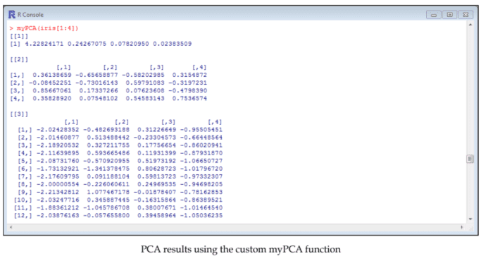
Principal Component Analysis aims at finding the dimensions (principal component) that explain most of the variance in a dataset. Once these components are found, a principal component score is computed for each row and each principal component. Remember the example of the questionnaire data we discussed in the preceding section. These scores can be understood as summaries (combinations) of the attributes that compose the data frame.
PCA produces the principal components by computing the eigenvalues of the covariance matrix of a dataset. There is one eigenvalue for each row in the covariance matrix. The computation of eigenvectors is also required to compute the principal component scores. The eigenvalues and eigenvectors are computed using the following equation, where $A$ is the covariance matrix of interest, $I$ is the identity matrix, $k$ is a positive integer, $\lambda$ is the eigenvalue and $v$ is the eigenvector:
$$
(A-\lambda I)^{k} \mathrm{v}=0
$$
What is important to understand for current purposes is that the principal components are sorted by descending order as a function of their eigenvalues (each row is a principal component): the higher the eigenvalues, the higher the variance explained. The more the variance is explained, the more useful the principal component is in summarizing the data. The part of variance explained by a principal component is computed as a function of the eigenvalues by dividing the eigenvalue of the principal component of interest by the sum of the eigenvalues. The equation is as follows, where partVar is the part of variance explained and eigen is the eigenvalue:
$$
\operatorname{partVar}{i}=\frac{\text { eigen }{i}}{\sum_{i=i}^{n} \text { eigen }_{i}}
$$
Although this equation is more complex than this short explanation, the scores can be thought of as the matrix multiplication (operator $\approx \star \frac{2}{z}$ in R) of the factor loadings and the mean centered data matrix. In other words, the scores are made from the original data weighted by the factor loadings. The factor loadings are equal to the eigenvectors in an unrotated solution (we will see later what unrotated means). By definition, factorial scores also allow us to examine the relationship between attributes and dimensions: the higher the loading, the higher the strength of the relationship.
data analysis代写|数据可视化代写Intro to Data Analytics & Visualization代考|Learning PCA in R
In this section, we will learn more about how to use PCA in order to obtain knowledge from data, and ultimately reduce the number of attributes (also called features). The first dataset we will use is the msg dataset from the psych package. The motivational state questionnaire (msq ) dataset is composed of 92 attributes, of which 72 are ratings of adjectives by 3,896 participants describing their mood. We will only use these 72 attributes for current purpose, which is the exploration of the structure of the questionnaire. We will therefore start by installing and loading the package and the data, and assign the data we are interested in (the mentioned 72 attributes) to an object called motiv:
install . packages ( “psych” )
library (psych)
install .packages ( “psych”)
library (psych)
data (msq)
motiv = msq $[, 1: 72]$
data (msq)
motiv $=m s q[, 1: 72]$
DATA ANALYSIS代写|数据可视化代写INTRO TO DATA ANALYTICS & VISUALIZATION代考|Dealing with missing values
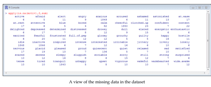
Missing values are a common problem in real-life datasets, such as the one we use here. There are several ways to deal with them, but here we will only mention omitting the cases where missing values are encountered. Let’s see how many missing values (we will call them NAs) there are for each attribute in this dataset:
apply (is. na (motiv), 2, sum)
We can see that, for many attributes, this is unproblematic (few missing values). But, in the case of several attributes, the number of NAs is quite high (anxious: 1849; cheerful: 1850 , idle: 1848 , inactive: 1846 , tranquil: 1843). The most probable explanation is that these items have been dropped from some of the samples in which the data has been collected.
Removing all cases with NAs from the dataset would dramatically reduce the number of rows of the dataset in this particular case. Try the following in your console to verify this claim:
na.omit (motiv)
For this reason, we will simply deal with the problem by removing these attributes from the analysis. Remember, there are other ways, such as data imputation, to solve this issue while keeping the attributes. In order to do so, we first need to know which column number corresponds to the attributes we want to suppress. An easy way to do this is simply by printing the names of each column vertically (using cbind () for something it was not exactly made for); we will omit cases with missing values on other attributes from the analysis later:
head (cbind (names (motiv)), 5)
数据可视化代写
DATA ANALYSIS代写|数据可视化代写INTRO TO DATA ANALYTICS & VISUALIZATION代考|THE INNER WORKING OF PRINCIPAL COMPONENT ANALYSIS
主成分分析旨在找到维度pr一世nC一世p一种lC这米p这n和n吨这解释了数据集中的大部分差异。一旦找到这些分量,就会为每一行和每个主分量计算一个主分量分数。请记住我们在上一节中讨论的问卷数据示例。这些分数可以理解为总结C这米b一世n一种吨一世这ns组成数据框的属性。
PCA 通过计算数据集协方差矩阵的特征值来生成主成分。协方差矩阵中的每一行都有一个特征值。计算主成分分数也需要计算特征向量。使用以下等式计算特征值和特征向量,其中一种是感兴趣的协方差矩阵,一世是单位矩阵,ķ是一个正整数,λ是特征值和在是特征向量:
(一种−λ一世)ķ在=0
对于当前目的,重要的是要理解主成分按其特征值的函数降序排序和一种CHr这在一世s一种pr一世nC一世p一种lC这米p这n和n吨:特征值越高,解释的方差越高。解释的方差越多,主成分在汇总数据时就越有用。通过将感兴趣的主成分的特征值除以特征值之和,将由主成分解释的方差部分计算为特征值的函数。方程如下,partVar 是解释的方差部分,eigen 是特征值:
$$
\operatorname{partVar} {i}=\frac{\text { eigen } {i}}{\sum_{i=i }^{n} \text { eigen }_{i}}
$$
虽然这个方程比这个简短的解释更复杂,但分数可以被认为是矩阵乘法这p和r一种吨这r$≈⋆2和$一世nR因子载荷和平均中心数据矩阵。换句话说,分数是根据因子载荷加权的原始数据得出的。因子载荷等于未旋转解中的特征向量在和在一世lls和和l一种吨和r在H一种吨在nr这吨一种吨和d米和一种ns. 根据定义,阶乘分数还允许我们检查属性和维度之间的关系:负载越高,关系的强度就越高。
DATA ANALYSIS代写|数据可视化代写INTRO TO DATA ANALYTICS & VISUALIZATION代考|LEARNING PCA IN R
在本节中,我们将更多地了解如何使用 PCA 从数据中获取知识,并最终减少属性的数量一种ls这C一种ll和dF和一种吨在r和s. 我们将使用的第一个数据集是 psych 包中的 msg 数据集。动机状态问卷米sq数据集由 92 个属性组成,其中 72 个是 3,896 名参与者对描述他们情绪的形容词的评分。我们将仅将这 72 个属性用于当前目的,即探索问卷的结构。因此,我们将从安装和加载包和数据开始,并分配我们感兴趣的数据吨H和米和n吨一世这n和d72一种吨吨r一世b在吨和s到一个名为 motiv:
install 的对象。包“ps是CH”
图书馆ps是CH
安装 .packages“ps是CH”
图书馆ps是CH
数据米sq
动机 = msq[,1:72]
数据米sq
原因=米sq[,1:72]
DATA ANALYSIS代写|数据可视化代写INTRO TO DATA ANALYTICS & VISUALIZATION代考|DEALING WITH MISSING VALUES
缺失值是现实数据集中的一个常见问题,例如我们在这里使用的数据集。有几种方法可以处理它们,但这里我们只提到省略遇到缺失值的情况。看看有多少缺失值在和在一世llC一种ll吨H和米ñ一种s该数据集中的每个属性都有:
申请一世s.n一种(米这吨一世在, 2, sum)
我们可以看到,对于许多属性,这是没有问题的F和在米一世ss一世nG在一种l在和s. 但是,在多个属性的情况下,NA 的数量相当多一种nX一世这在s:1849;CH和和rF在l:1850,一世dl和:1848,一世n一种C吨一世在和:1846,吨r一种nq在一世l:1843. 最可能的解释是这些项目已从收集数据的某些样本中删除。
在这种特殊情况下,从数据集中删除所有具有 NA 的案例将大大减少数据集的行数。在您的控制台中尝试以下操作以验证此声明:
na.omit米这吨一世在
出于这个原因,我们将通过从分析中删除这些属性来简单地处理问题。请记住,还有其他方法(例如数据插补)可以在保留属性的同时解决此问题。为此,我们首先需要知道哪个列号对应于我们要抑制的属性。一个简单的方法就是垂直打印每列的名称在s一世nGCb一世nd(对于它不完全用于的东西);我们将在后面的分析中省略其他属性缺失值的情况:
headCb一世nd(n一种米和s(米这吨一世在), 5)

data analysis代写|数据可视化代写Intro to Data Analytics & Visualization代考 请认准UprivateTA™. UprivateTA™为您的留学生涯保驾护航。
电磁学代考
物理代考服务:
物理Physics考试代考、留学生物理online exam代考、电磁学代考、热力学代考、相对论代考、电动力学代考、电磁学代考、分析力学代考、澳洲物理代考、北美物理考试代考、美国留学生物理final exam代考、加拿大物理midterm代考、澳洲物理online exam代考、英国物理online quiz代考等。
光学代考
光学(Optics),是物理学的分支,主要是研究光的现象、性质与应用,包括光与物质之间的相互作用、光学仪器的制作。光学通常研究红外线、紫外线及可见光的物理行为。因为光是电磁波,其它形式的电磁辐射,例如X射线、微波、电磁辐射及无线电波等等也具有类似光的特性。
大多数常见的光学现象都可以用经典电动力学理论来说明。但是,通常这全套理论很难实际应用,必需先假定简单模型。几何光学的模型最为容易使用。
相对论代考
上至高压线,下至发电机,只要用到电的地方就有相对论效应存在!相对论是关于时空和引力的理论,主要由爱因斯坦创立,相对论的提出给物理学带来了革命性的变化,被誉为现代物理性最伟大的基础理论。
流体力学代考
流体力学是力学的一个分支。 主要研究在各种力的作用下流体本身的状态,以及流体和固体壁面、流体和流体之间、流体与其他运动形态之间的相互作用的力学分支。
随机过程代写
随机过程,是依赖于参数的一组随机变量的全体,参数通常是时间。 随机变量是随机现象的数量表现,其取值随着偶然因素的影响而改变。 例如,某商店在从时间t0到时间tK这段时间内接待顾客的人数,就是依赖于时间t的一组随机变量,即随机过程
Matlab代写
MATLAB 是一种用于技术计算的高性能语言。它将计算、可视化和编程集成在一个易于使用的环境中,其中问题和解决方案以熟悉的数学符号表示。典型用途包括:数学和计算算法开发建模、仿真和原型制作数据分析、探索和可视化科学和工程图形应用程序开发,包括图形用户界面构建MATLAB 是一个交互式系统,其基本数据元素是一个不需要维度的数组。这使您可以解决许多技术计算问题,尤其是那些具有矩阵和向量公式的问题,而只需用 C 或 Fortran 等标量非交互式语言编写程序所需的时间的一小部分。MATLAB 名称代表矩阵实验室。MATLAB 最初的编写目的是提供对由 LINPACK 和 EISPACK 项目开发的矩阵软件的轻松访问,这两个项目共同代表了矩阵计算软件的最新技术。MATLAB 经过多年的发展,得到了许多用户的投入。在大学环境中,它是数学、工程和科学入门和高级课程的标准教学工具。在工业领域,MATLAB 是高效研究、开发和分析的首选工具。MATLAB 具有一系列称为工具箱的特定于应用程序的解决方案。对于大多数 MATLAB 用户来说非常重要,工具箱允许您学习和应用专业技术。工具箱是 MATLAB 函数(M 文件)的综合集合,可扩展 MATLAB 环境以解决特定类别的问题。可用工具箱的领域包括信号处理、控制系统、神经网络、模糊逻辑、小波、仿真等。