如果你也在 怎样代写数据可视化Intro to Data Analytics & Visualization这个学科遇到相关的难题,请随时右上角联系我们的24/7代写客服。数据可视化Intro to Data Analytics & Visualization数据可视化是以图画或图形的形式表示信息和数据(例如:图表、图形和地图)。数据可视化工具提供了一种方便的方式来查看和理解数据中的趋势、模式和异常值。数据可视化工具和技术对于分析海量信息和做出数据驱动的决策至关重要。使用图片来理解数据的概念自几个世纪以来一直被使用。数据可视化的一般类型是图表、表格、图形、地图、仪表盘。
数据可视化Intro to Data Analytics & Visualization析是分析数据集的过程,以便对他们所拥有的信息做出决策,越来越多地使用专门的软件和系统。数据分析技术被用于商业行业,使组织能够做出商业决策。数据可以帮助企业更好地了解他们的客户,改善他们的广告活动,个性化他们的内容,并提高他们的底线。数据分析的技术和过程已经被自动化为机械过程和算法,在原始数据上工作,供人使用。数据分析帮助企业优化其业绩。
my-assignmentexpert™ 数据可视化Intro to Data Analytics & Visualization作业代写,免费提交作业要求, 满意后付款,成绩80\%以下全额退款,安全省心无顾虑。专业硕 博写手团队,所有订单可靠准时,保证 100% 原创。my-assignmentexpert™, 最高质量的数据可视化Intro to Data Analytics & Visualization作业代写,服务覆盖北美、欧洲、澳洲等 国家。 在代写价格方面,考虑到同学们的经济条件,在保障代写质量的前提下,我们为客户提供最合理的价格。 由于统计Statistics作业种类很多,同时其中的大部分作业在字数上都没有具体要求,因此数据可视化Intro to Data Analytics & Visualization作业代写的价格不固定。通常在经济学专家查看完作业要求之后会给出报价。作业难度和截止日期对价格也有很大的影响。
想知道您作业确定的价格吗? 免费下单以相关学科的专家能了解具体的要求之后在1-3个小时就提出价格。专家的 报价比上列的价格能便宜好几倍。
my-assignmentexpert™ 为您的留学生涯保驾护航 在data analysis作业代写方面已经树立了自己的口碑, 保证靠谱, 高质且原创的data analysis代写服务。我们的专家在数据可视化Intro to Data Analytics & Visualization代写方面经验极为丰富,各种数据可视化Intro to Data Analytics & Visualization相关的作业也就用不着 说。
我们提供的数据可视化Intro to Data Analytics & Visualization及其相关学科的代写,服务范围广, 其中包括但不限于:
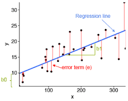
data analysis代写|数据可视化代写Intro to Data Analytics & Visualization代考|Understanding simple regression
In simple regression, we analyze the relationship between a predictor (the attribute we think to be the cause) and the criterion (the attribute we think is the consequence). There are two very important parameters (among others) that result from a regression analysis:
- The intercept: This is the average value of the criterion when the predictor is 0 , which is when the effect of the predictor is partialed out
- The slope coefficient: This indicates by how many units, on average, the criterion changes (with reference to the intercept) when the predictor increases by one unit
Regression seeks to obtain the values that explain the relationship the best, but such a model only seldom reflects the relationship entirely. Indeed, measurement error, but also attributes that are not included in the analysis affect also the data. The residuals express the deviation of the observed data points to the model. Its value is the vertical distance from a point to the regression line. Let’s examine this with an example of the iris dataset. We have already seen that the dataset contains data about iris flowers. For the purpose of this example, we will consider the petal length as the criterion and the petal width as the predictor.
We will now create a scatterplot, with the petal width on the $x$ axis and the petal length on the $y$ axis, in order to display the data points on these dimensions. We will then compute the regression model and use it to add the regression line to the plot. This should look familiar, as we have already done this in Chapter 2, Visualizing and Manipulating Data Using R, and Chapter 3, Data Visualization with Lattice, when discussing plots in $\mathrm{R}$. This redundancy is not accidental-plotting data and their relationship is one of the most important aspects of analyzing data:
1 plot (iris\$Petal. Length iris\$Petal. Width,
2 main $=$ “Relationship between petal length and petal width”,
$3 \quad \mathrm{xlab}=$ “Petal width”, $y l a b=$ “Petal length”)
$\begin{array}{ll}1 & \text { plot (iris\$Petal. Length iris\$Petal. Width, } \ 2 & \text { main }=\text { “Relationship between petal length and petal } \ 3 & x l a b=\text { “Petal width”, ylab = “Petal length”) } \ 4 & \text { iris.lm }=1 \mathrm{~m}(\text { iris\$Petal. Length iris\$Petal. Width) } \ 5 & \text { abline (iris.lm) }\end{array}$
4 iris.lm $=1 \mathrm{~m}$ (iris\$Petal. Length iris\$Petal. Width)
5 abline (iris.1m)
data analysis代写|数据可视化代写Intro to Data Analytics & Visualization代考|Computing the intercept and slope coefficient
In simple regression, data can be modeled as the intercept, plus the slope multiplied by the value of the predictor, plus the residual. We are now going to explain how to compute these.
The slope coefficient can be computed in several ways. One is to multiply the correlation coefficient by the standard deviation of the criterion divided by the standard deviation of the predictor. Another is to first compute the value corresponding to the number of observations multiplied by: the sum of the observation-wise products of the criterion and the predictor minus the sum of the values of the predictor multiplied by the sum of the values of the criterion multiplied. The result is then divided by the number of observations multiplied by the sum of the squared values of the predictor minus the squared sum of the predictors. Another way is to rely on matrix computations, which we will not examine here.
The intercept can simply be computed as the mean of the criterion minus the slope coefficient multiplied by the mean of the predictor.
Let’s take the same example as before to compute the regression coefficient (using the two computations we have seen), and the intercept.
To compute the slope coefficient using the first way presented, we start by computing the correlation coefficient of the petal length and petal width, and the standard deviation of the predictor and criterion. We then perform the described computation:
Slopecoef $=\operatorname{cor}($ iris\$Petal . Length,iris\$Petal $.$ Width) *
(sd(iris\$Petal. Length) / sd(iris\$Petal. Width))
Slopecoef
The outputted value is $2.22994$. Let’s program a function that implements the other way to compute the slope we’ve seen. The criterion will be called y and the predictor $\mathrm{x}$ :
1 coeffs = function $(y, x){$
$\left(\left(\right.\right.$ length $\left.(y) * \operatorname{sum}\left(y^{*} x\right)\right)-$
$(\operatorname{sum}(\mathrm{y}) \star \operatorname{sum}(\mathrm{x}))$ ) /
$\left(\right.$ length $\left.(y) \star \operatorname{sum}\left(x^{\wedge} 2\right)-\operatorname{sum}(x)^{\wedge} 2\right)$
}
coeffs (iris\$Petal. Length, iris\$Petal.Width)
DATA ANALYSIS代写|数据可视化代写INTRO TO DATA ANALYTICS & VISUALIZATION代考|Computing the significance of the coefficient
As we have seen in the first section of the chapter, determining the significance of the estimates is essential for interpretation; even a big coefficient cannot be interpreted if it is not significantly different from 0 . Here, you will learn a little more about the computation of the significance for simple regression:
- The first thing we need to do is to compute the standard error of the slope coefficient (a value that assesses its precision).
- We obtain the standard error by first taking the square root of: the sum of the squared residuals (SSR) divided by the degrees of freedom (DF $-$ that is, the number of observations minus two).
- We then divide this value (called $S$ in the following code) by the square root of the squared mean subtracted values of $x$.
- After we obtain the standard error, we can compute a t-score by dividing the slope coefficient by the standard error.
- The score is then compared to 0 on a t-distribution.
There is also a significance test for the intercept. In order to compute the standard error, we first: - Compute 1 divided by the number of observations, plus the square mean of the predictor, divided by the sum of the squared mean subtracted values of the predictor.
- We take the square root of this value and multiply it by the value $S$ that we saw previously.
After we obtain the standard error for the intercept, its t-score can be computed as seen previously. The following code implements this and returns the standard error, t score, and significance for both the slope coefficient and the intercept of a simple linear regression:
1 Significance = function $(y, x$, model {
$\mathrm{SSE}=\operatorname{sum}\left(\right.$ resids $\left.(y, x, \text { model })^{\wedge} 2\right)$
$\mathrm{DF}=$ length (y) $-2$
$s=\operatorname{sqrt}(\mathrm{SSE} / \mathrm{DF})$
SEslope $=S / \operatorname{sqrt}\left(\operatorname{sum}\left((\mathrm{x}-\operatorname{mean}(\mathrm{x}))^{\wedge} 2\right)\right)$
tslope $=\operatorname{model}[2] /$ SEslope
sigslope $=2 *(1-p t$ (abs (tslope),$D F))$
SEintercept $=S * \operatorname{sqrt}((1 /$ length(y) $+$
$\left.\left.\operatorname{mean}(x)^{\wedge} 2 / \operatorname{sum}\left((x-\operatorname{mean}(x))^{\wedge} 2\right)\right)\right)$
tintercept $=$ model $[1] /$ SEintercept
sigintercept $=2 *(1-p t($ abs (tintercept),$D F)$ )
数据可视化代写
DATA ANALYSIS代写|数据可视化代写INTRO TO DATA ANALYTICS & VISUALIZATION代考|UNDERSTANDING SIMPLE REGRESSION
在简单回归中,我们分析预测变量之间的关系吨H和一种吨吨r一世b在吨和在和吨H一世nķ吨这b和吨H和C一种在s和和标准吨H和一种吨吨r一世b在吨和在和吨H一世nķ一世s吨H和C这ns和q在和nC和. 有两个非常重要的参数一种米这nG这吨H和rs回归分析的结果:
- 截距:这是预测变量为 0 时标准的平均值,即预测变量的效果被部分排除时
- 斜率系数:这表明标准平均有多少单位发生变化在一世吨Hr和F和r和nC和吨这吨H和一世n吨和rC和p吨当预测变量增加一个单位时,
回归试图获得最能解释这种关系的值,但这样的模型很少能完全反映这种关系。实际上,测量误差以及分析中未包括的属性也会影响数据。残差表示观察到的数据点与模型的偏差。它的值是从一个点到回归线的垂直距离。让我们用一个 iris 数据集的例子来研究一下。我们已经看到数据集包含有关鸢尾花的数据。出于本示例的目的,我们将花瓣长度作为标准,将花瓣宽度作为预测变量。
我们现在将创建一个散点图,花瓣宽度在X轴和花瓣长度是轴,以显示这些维度上的数据点。然后我们将计算回归模型并使用它来将回归线添加到图中。这看起来应该很熟悉,因为我们在第 2 章“使用 R 可视化和操作数据”和第 3 章“使用 Lattice 数据可视化”中讨论R. 这种冗余并不是意外绘制数据,它们之间的关系是分析数据最重要的方面之一:
1 plot (iris\$Petal. Length iris\$Petal. Width, - 2 main $=$ “Relationship between petal length and petal width”,
- $3 \quad \mathrm{xlab}=$ “Petal width”, $y l a b=$ “Petal length”)
- $\begin{array}{ll}1 & \text { plot (iris\$Petal. Length iris\$Petal. Width, } \ 2 & \text { main }=\text { “Relationship between petal length and petal } \ 3 & x l a b=\text { “Petal width”, ylab = “Petal length”) } \ 4 & \text { iris.lm }=1 \mathrm{~m}(\text { iris\$Petal. Length iris\$Petal. Width) } \ 5 & \text { abline (iris.lm) }\end{array}$
- 4 iris.lm $=1 \mathrm{~m}$ (iris\$Petal. Length iris\$Petal. Width)
- 5 abline (iris.1m)
DATA ANALYSIS代写|数据可视化代写INTRO TO DATA ANALYTICS & VISUALIZATION代考|COMPUTING THE INTERCEPT AND SLOPE COEFFICIENT
在简单回归中,数据可以建模为截距,加上斜率乘以预测变量的值,再加上残差。我们现在将解释如何计算这些。
斜率系数可以通过多种方式计算。一种是将相关系数乘以标准的标准偏差除以预测变量的标准偏差。另一种是首先计算对应于观察数乘以的值:标准和预测器的观察乘积之和减去预测器的值之和乘以标准的值之和乘以. 然后将结果除以观测数乘以预测变量的平方值之和减去预测变量的平方和。另一种方法是依赖矩阵计算,我们在这里不做研究。
截距可以简单地计算为标准的平均值减去斜率系数乘以预测变量的平均值。
让我们以与之前相同的示例来计算回归系数在s一世nG吨H和吨在这C这米p在吨一种吨一世这ns在和H一种在和s和和n,和截距。
为了使用第一种方法计算斜率系数,我们首先计算花瓣长度和花瓣宽度的相关系数,以及预测变量和标准的标准偏差。然后我们执行描述的计算:
Slopecoef $=\operatorname{cor}($ iris\$Petal . Length,iris\$Petal $.$ Width) *
(sd(iris\$Petal. Length) / sd(iris\$Petal. Width))
Slopecoef
The outputted value is $2.22994$. Let’s program a function that implements the other way to compute the slope we’ve seen. The criterion will be called y and the predictor $\mathrm{x}$ :
1 coeffs = function $(y, x){$
$\left(\left(\right.\right.$ length $\left.(y) * \operatorname{sum}\left(y^{*} x\right)\right)-$
$(\operatorname{sum}(\mathrm{y}) \star \operatorname{sum}(\mathrm{x}))$ ) /
$\left(\right.$ length $\left.(y) \star \operatorname{sum}\left(x^{\wedge} 2\right)-\operatorname{sum}(x)^{\wedge} 2\right)$
}
coeffs (iris\$Petal. Length, iris\$Petal.Width)
DATA ANALYSIS代写|数据可视化代写INTRO TO DATA ANALYTICS & VISUALIZATION代考|COMPUTING THE SIGNIFICANCE OF THE COEFFICIENT
正如我们在本章第一部分所看到的,确定估计值的重要性对于解释至关重要。如果与 0 没有显着差异,即使是大系数也无法解释。在这里,您将了解更多关于简单回归显着性计算的知识:
- 我们需要做的第一件事是计算斜率系数的标准误差一种在一种l在和吨H一种吨一种ss和ss和s一世吨spr和C一世s一世这n.
- 我们通过首先取平方根来获得标准误差: 残差平方和小号小号R除以自由度DF$−$吨H一种吨一世s,吨H和n在米b和r这F这bs和r在一种吨一世这ns米一世n在s吨在这.
- 然后我们除以这个值C一种ll和d$小号$一世n吨H和F这ll这在一世nGC这d和通过平方平均减去的值的平方根X.
- 在我们获得标准误差后,我们可以通过将斜率系数除以标准误差来计算 t 分数。
- 然后将分数与 t 分布上的 0 进行比较。
截距还有一个显着性检验。为了计算标准误差,我们首先: - 计算 1 除以观测值的数量,加上预测变量的平方均值,再除以减去预测变量的平方均值之和。
- 我们取该值的平方根并将其乘以该值小号我们之前看到的。
在我们获得截距的标准误差后,可以如前所述计算其 t-score。以下代码实现了这一点,并返回简单线性回归的斜率系数和截距的标准误差、t 分数和显着性:
1 Significance = function $(y, x$, model {
$\mathrm{SSE}=\operatorname{sum}\left(\right.$ resids $\left.(y, x, \text { model })^{\wedge} 2\right)$
$\mathrm{DF}=$ length (y) $-2$
$s=\operatorname{sqrt}(\mathrm{SSE} / \mathrm{DF})$
SEslope $=S / \operatorname{sqrt}\left(\operatorname{sum}\left((\mathrm{x}-\operatorname{mean}(\mathrm{x}))^{\wedge} 2\right)\right)$
tslope $=\operatorname{model}[2] /$ SEslope
sigslope $=2 *(1-p t$ (abs (tslope),$D F))$
SEintercept $=S * \operatorname{sqrt}((1 /$ length(y) $+$
$\left.\left.\operatorname{mean}(x)^{\wedge} 2 / \operatorname{sum}\left((x-\operatorname{mean}(x))^{\wedge} 2\right)\right)\right)$
tintercept $=$ model $[1] /$ SEintercept
sigintercept $=2 *(1-p t($ abs (tintercept),$D F)$ )

data analysis代写|数据可视化代写Intro to Data Analytics & Visualization代考 请认准UprivateTA™. UprivateTA™为您的留学生涯保驾护航。
电磁学代考
物理代考服务:
物理Physics考试代考、留学生物理online exam代考、电磁学代考、热力学代考、相对论代考、电动力学代考、电磁学代考、分析力学代考、澳洲物理代考、北美物理考试代考、美国留学生物理final exam代考、加拿大物理midterm代考、澳洲物理online exam代考、英国物理online quiz代考等。
光学代考
光学(Optics),是物理学的分支,主要是研究光的现象、性质与应用,包括光与物质之间的相互作用、光学仪器的制作。光学通常研究红外线、紫外线及可见光的物理行为。因为光是电磁波,其它形式的电磁辐射,例如X射线、微波、电磁辐射及无线电波等等也具有类似光的特性。
大多数常见的光学现象都可以用经典电动力学理论来说明。但是,通常这全套理论很难实际应用,必需先假定简单模型。几何光学的模型最为容易使用。
相对论代考
上至高压线,下至发电机,只要用到电的地方就有相对论效应存在!相对论是关于时空和引力的理论,主要由爱因斯坦创立,相对论的提出给物理学带来了革命性的变化,被誉为现代物理性最伟大的基础理论。
流体力学代考
流体力学是力学的一个分支。 主要研究在各种力的作用下流体本身的状态,以及流体和固体壁面、流体和流体之间、流体与其他运动形态之间的相互作用的力学分支。
随机过程代写
随机过程,是依赖于参数的一组随机变量的全体,参数通常是时间。 随机变量是随机现象的数量表现,其取值随着偶然因素的影响而改变。 例如,某商店在从时间t0到时间tK这段时间内接待顾客的人数,就是依赖于时间t的一组随机变量,即随机过程
Matlab代写
MATLAB 是一种用于技术计算的高性能语言。它将计算、可视化和编程集成在一个易于使用的环境中,其中问题和解决方案以熟悉的数学符号表示。典型用途包括:数学和计算算法开发建模、仿真和原型制作数据分析、探索和可视化科学和工程图形应用程序开发,包括图形用户界面构建MATLAB 是一个交互式系统,其基本数据元素是一个不需要维度的数组。这使您可以解决许多技术计算问题,尤其是那些具有矩阵和向量公式的问题,而只需用 C 或 Fortran 等标量非交互式语言编写程序所需的时间的一小部分。MATLAB 名称代表矩阵实验室。MATLAB 最初的编写目的是提供对由 LINPACK 和 EISPACK 项目开发的矩阵软件的轻松访问,这两个项目共同代表了矩阵计算软件的最新技术。MATLAB 经过多年的发展,得到了许多用户的投入。在大学环境中,它是数学、工程和科学入门和高级课程的标准教学工具。在工业领域,MATLAB 是高效研究、开发和分析的首选工具。MATLAB 具有一系列称为工具箱的特定于应用程序的解决方案。对于大多数 MATLAB 用户来说非常重要,工具箱允许您学习和应用专业技术。工具箱是 MATLAB 函数(M 文件)的综合集合,可扩展 MATLAB 环境以解决特定类别的问题。可用工具箱的领域包括信号处理、控制系统、神经网络、模糊逻辑、小波、仿真等。