如果你也在 怎样代写量子力学Quantum mechanics这个学科遇到相关的难题,请随时右上角联系我们的24/7代写客服。量子力学Quantum mechanics在理论物理学中,量子场论(QFT)是一个结合了经典场论、狭义相对论和量子力学的理论框架。QFT在粒子物理学中用于构建亚原子粒子的物理模型,在凝聚态物理学中用于构建准粒子的模型。
量子力学Quantum mechanics产生于跨越20世纪大部分时间的几代理论物理学家的工作。它的发展始于20世纪20年代对光和电子之间相互作用的描述,最终形成了第一个量子场理论–量子电动力学。随着微扰计算中各种无限性的出现和持续存在,一个主要的理论障碍很快出现了,这个问题直到20世纪50年代随着重正化程序的发明才得以解决。第二个主要障碍是QFT显然无法描述弱相互作用和强相互作用,以至于一些理论家呼吁放弃场论方法。20世纪70年代,规整理论的发展和标准模型的完成导致了量子场论的复兴。
量子力学Quantum mechanics代写,免费提交作业要求, 满意后付款,成绩80\%以下全额退款,安全省心无顾虑。专业硕 博写手团队,所有订单可靠准时,保证 100% 原创。最高质量的量子力学Quantum mechanics作业代写,服务覆盖北美、欧洲、澳洲等 国家。 在代写价格方面,考虑到同学们的经济条件,在保障代写质量的前提下,我们为客户提供最合理的价格。 由于作业种类很多,同时其中的大部分作业在字数上都没有具体要求,因此量子力学Quantum mechanics作业代写的价格不固定。通常在专家查看完作业要求之后会给出报价。作业难度和截止日期对价格也有很大的影响。
同学们在留学期间,都对各式各样的作业考试很是头疼,如果你无从下手,不如考虑my-assignmentexpert™!
my-assignmentexpert™提供最专业的一站式服务:Essay代写,Dissertation代写,Assignment代写,Paper代写,Proposal代写,Proposal代写,Literature Review代写,Online Course,Exam代考等等。my-assignmentexpert™专注为留学生提供Essay代写服务,拥有各个专业的博硕教师团队帮您代写,免费修改及辅导,保证成果完成的效率和质量。同时有多家检测平台帐号,包括Turnitin高级账户,检测论文不会留痕,写好后检测修改,放心可靠,经得起任何考验!
想知道您作业确定的价格吗? 免费下单以相关学科的专家能了解具体的要求之后在1-3个小时就提出价格。专家的 报价比上列的价格能便宜好几倍。
我们在物理Physical代写方面已经树立了自己的口碑, 保证靠谱, 高质且原创的物理Physical代写服务。我们的专家在量子力学Quantum mechanics代写方面经验极为丰富,各种量子力学Quantum mechanics相关的作业也就用不着说。
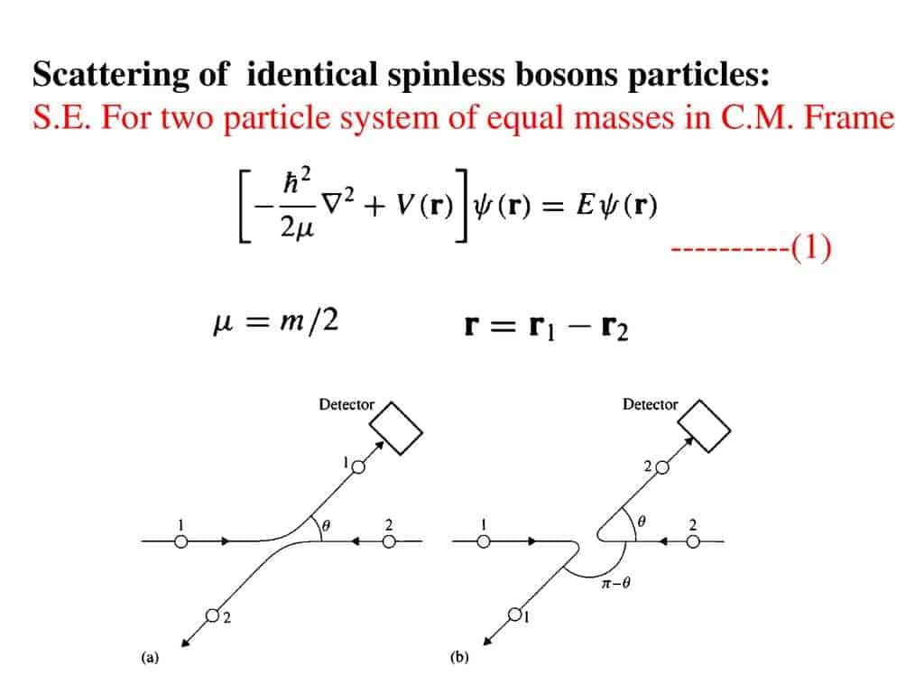
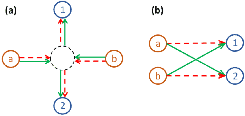
物理代写|量子力学代写Quantum mechanics代考|Scattering of identical particles
Consider two identical particles that are scattered by a finite range potential $V(\mathbf{r})$. The total wavefunction $\Psi\left(\mathbf{r}1, \mathbf{r}_2\right)$ can be written in terms of the center of mass and relative coordinates $\mathbf{R}$ and $\mathbf{r}$ respectively. In this basis the wavefunction is separable $$ \Psi\left(\mathbf{r}_1, \mathbf{r}_2\right)=\Psi(\mathbf{R}, \mathbf{r})=\Psi{c m}(\mathbf{R}) \Psi_{r e l}(\mathbf{r})
$$
Since $\Psi_{c m}(\mathbf{R})$ is trivial we concentrate on $\Psi_{r e l}(\mathbf{r})$ and for simplicity rename it $\Psi(\mathbf{r})$
Allowing for spin degrees of freedom, each wavefunction has an additional spin index to represent an appropriate spinning wavefunction. Therefore the two particle wavefunction has a pair of spin indices, and is denoted as $\Psi_{\sigma_1, \sigma_2}(\mathbf{r})$. Under the interchange of two identical particles this wavefunction must satisfy quantum statistics.
First we consider spinless bosons. There are no spin indices and the wavefunction must be even under the interchange of the positions of the two particles. For the relative wavefunction this amounts to
Spinless bosons: $\Psi(\mathbf{r})=\Psi(-\mathbf{r})$
Hence the wave function for scattered particles must have the form
$$
\begin{aligned}
\Psi_{\mathbf{k}}(\mathbf{r}) & =\frac{C}{(2 \pi)^{3 / 2}}\left[\left(e^{i \mathbf{k} \cdot \mathbf{r}}+e^{-i \mathbf{k} \cdot \mathbf{r}}\right)+\frac{e^{i k r}}{r}(f(\mathbf{k}, \hat{\mathbf{r}})+f(\mathbf{k},-\hat{\mathbf{r}}))\right] \
& =\frac{C}{(2 \pi)^{3 / 2}}\left[\left(e^{i \mathbf{k} \cdot \mathbf{r}}+e^{-i \mathbf{k} \cdot \mathbf{r}}\right)+\frac{e^{i k r}}{r}(f(E, \theta)+f(E, \pi-\theta))\right]
\end{aligned}
$$
where we have used $f(\mathbf{k}, \hat{\mathbf{r}})=f(E, \theta)$.
物理代写|量子力学代写Quantum mechanics代考|Born approximation
We have seen that the differential cross section $d \sigma$ is directly proportional to $\left|f\left(\mathbf{k}, \mathbf{k}^{\prime}\right)\right|^2$, which, in turn, was expressed as $f\left(\mathbf{k}, \mathbf{k}^{\prime}\right)=-2 \pi^2\left\langle\mathbf{k}^{\prime}|v(r)| \mathbf{k}\right\rangle^{+}$. Scattering experiments then give us a possibility to discover the matrix elements of $V(r)$ in momentum space thus revealing the properties of the interaction $V(r)$. This property is particularly evident in the First Born Approximation denoted as $f^{(1)}\left(\mathbf{k}, \mathbf{k}^{\prime}\right)$, which corresponds to approximating the state $|\mathbf{k}\rangle^{+}$with the free particle state $|\mathbf{k}\rangle$. We will later investigate the conditions under which the approximation is valid. In this case indeed $f^{(1)}\left(\mathbf{k}, \mathbf{k}^{\prime}\right)$ is proportional to the matrix elements of $V(r)$ in the free particle Hilbert space $\left\langle\mathbf{k}^{\prime}|V(r)| \mathbf{k}\right\rangle$ which is given by representing the states with plane waves as in Eq.(14.3)
$$
f^{(1)}\left(\mathbf{k}^{\prime}, \mathbf{k}\right)=-2 \pi^2 \int d^3 \mathbf{r} \frac{e^{-i \mathbf{k}^{\prime} \cdot \mathbf{r}}}{(2 \pi)^{3 / 2}} \frac{2 m}{\hbar^2} V(r) \frac{e^{i \mathbf{k} \cdot \mathbf{r}}}{(2 \pi)^{3 / 2}}
$$
This is just a Fourier transform of the potential using the momentum transfer $\hbar\left(\mathbf{k}^{\prime}-\mathbf{k}\right)$
$$
f^{(1)}\left(\mathbf{k}^{\prime}-\mathbf{k}\right)=-\frac{m}{2 \pi \hbar^2} \int d^3 \mathbf{r} V(r) e^{-i\left(\mathbf{k}^{\prime}-\mathbf{k}\right) \cdot \mathbf{r}}
$$
For a rotationally invariant potential this is a function of only $\left|\mathbf{k}^{\prime}-\mathbf{k}\right|=2 k \sin (\theta / 2)$. Thus, from the scattering amplitude one can extract the details of the potential $V(r)$ through the inverse Fourier transform. One can thus probe the scatterer by bombarding it with a beam of known particles and extract the nature of the forces between beam and target by measuring the energy and angle dependence of the differential cross section.
To justify the approximation we start from the general expression of the scattering amplitude $f\left(\mathbf{k}, \mathbf{k}^{\prime}\right)=-2 \pi^2\left\langle\mathbf{k}^{\prime}|v(r)| \mathbf{k}\right\rangle^{+}$, and the Lippmann-Schwinger equation $|\mathbf{k}\rangle^{+}=|\mathbf{k}\rangle+G v|\mathbf{k}\rangle^{+}$, where $G=\left(k^2-\mathbf{p}^2 / \hbar^2+i \varepsilon\right)^{-1}$ is the operator version of the Green function. We solve formally for $|\mathbf{k}\rangle^{+}$and substitute it in $f\left(\mathbf{k}, \mathbf{k}^{\prime}\right)$ to get the exact expressions
$$
|\mathbf{k}\rangle^{+}=(1-G v)^{-1}|\mathbf{k}\rangle, \quad f\left(\mathbf{k}, \mathbf{k}^{\prime}\right)=-2 \pi^2\left\langle\mathbf{k}^{\prime}\left|v(r)(1-G v)^{-1}\right| \mathbf{k}\right\rangle .
$$
量子力学代写
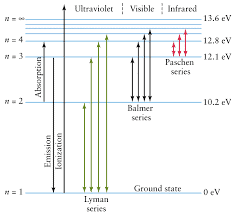
物理代写|量子力学代写QUANTUM MECHANICS代考|IONIZATION OF A HYDROGEN ATOM BY A RADIATION FIELD
考虑空间恒定的随时间变化的振荡电场中的 $\mathrm{H}$ 原子。标量势是 $A_0=-\mathbf{r} \cdot \mathbf{E}(t)$ 并且电子通过术语与电场相互作用 $-e A_0$ 在哈密顿量中。因此,对 于电场中 $z$ 扰动的方向
$$
H^{\prime}(t)=e \mathbf{r} \cdot \mathbf{E}(t)=e E(t) \mathbf{r} \cdot \hat{\mathbf{E}}
$$
我们将采取 $E(t)=E_0\left(e^{i \omega t}+e^{-i \omega t}\right)$, 然后选择一个方便的方向言对于电场。然后
$$
H^{\prime}(t)=A e^{i \omega t}+A^{\dagger} e^{-i \omega t}, A=e E_0 \mathbf{r} \cdot \hat{\mathbf{E}}
$$
根据上一节的计算,我们有
对于氢的电离,我们取初态为基态,而终态为具有动量的自由粒子态 $\mathbf{p}$. 因此我们需要计算
$$
\begin{aligned}
\langle f|A| i\rangle & =e E_0\langle\mathbf{p}|\mathbf{r} \cdot \hat{\mathbf{E}}| 100\rangle \mathbf{r}^{\prime} \
& =e E_0 \int d^3 \mathbf{r}^{\prime}\left\langle\mathbf{p} \mid \mathbf{r}^{\prime}\right\rangle r^{\prime} \mathbf{r}^{\prime} \cdot \hat{\mathbf{E}}\left\langle\mathbf{r}^{\prime} \mid 100\right\rangle \
& =e E_0 \int d^3 r \frac{1}{(L)^{3 / 2}} \exp \left(-\frac{i}{\hbar} \mathbf{p} \cdot \mathbf{r}^{\prime}\right) r^{\prime} \hat{\mathbf{r}}^{\prime} \cdot \hat{\mathbf{E}} \frac{e^{-r^{\prime} / a_0}}{\sqrt{\pi a_0^3}} \
& =\frac{e E_0}{\sqrt{\pi}\left(L a_0\right)^{3 / 2}} \int d^3 \mathbf{r}^{\prime} \exp \left(-\frac{i}{\hbar} \mathbf{p} \cdot \mathbf{r}^{\prime}\right) r^{\prime} \hat{\mathbf{r}}^{\prime} \cdot \hat{\mathbf{E}} e^{-r^{\prime} / a_0}
\end{aligned}
$$
物理代写|量子力学代写QUANTUM MECHANICS代考|LIPPMANN-SCHWINGER EQUATION
我们现在准备好解决入射自由动量粒子的典型散射问题 $\mathbf{p}=\hbar \mathbf{k}$ 与时间无关的潜力相互作用 $V(\mathbf{r})$. 这个过程是时间相关的,即使哈密顿量没有明确 地依赖于时间。哈密顿量是
$$
H=H_0+H^{\prime}=\frac{\mathbf{p}^2}{2 m}+V(\mathbf{r})
$$
目标是确定概率幅度 $\Psi_{\mathbf{k}}(\mathbf{r})$ 用于在某个位置找到传出粒子 $\mathbf{r}$ 入射粒子散射后。这些信息可以通过求解具有适当初始条件的薛定谔方程来获得。一种 方法是推导一个称为李普曼-施温格方程的积分方程,它等价于薛定谔方程并包含边界条件。
由于与时间无关的哈密顿量,在散射过程中能量守恒,因此我们必须匹配能量特征值 $H_0$ 和 $H$ 正如我们在上一章中学到的。自从 $H_0$ 管理传入状态 $|E\rangle$ ,尽管 $H$ 治国 $|E\rangle^{+}$在散射过程中,我们用相同的方式写出特征值方程 $E$
$$
H|E\rangle^{+}=E|E\rangle^{+}, \quad H_0|E\rangle=E|E\rangle
$$
正如我们在上一章中了解到的,李普曼-施温格方程描述了初始状态的演化 $|E\rangle$ 进入状态 $|E\rangle+$ 作为互动的结果
$$
|E\rangle^{+}=|E\rangle+\left(E-H_0+i \varepsilon\right)^{-1} H^{\prime}|E\rangle^{+}
$$

物理代写|量子力学代写Quantum mechanics代考 请认准UprivateTA™. UprivateTA™为您的留学生涯保驾护航。
微观经济学代写
微观经济学是主流经济学的一个分支,研究个人和企业在做出有关稀缺资源分配的决策时的行为以及这些个人和企业之间的相互作用。my-assignmentexpert™ 为您的留学生涯保驾护航 在数学Mathematics作业代写方面已经树立了自己的口碑, 保证靠谱, 高质且原创的数学Mathematics代写服务。我们的专家在图论代写Graph Theory代写方面经验极为丰富,各种图论代写Graph Theory相关的作业也就用不着 说。
线性代数代写
线性代数是数学的一个分支,涉及线性方程,如:线性图,如:以及它们在向量空间和通过矩阵的表示。线性代数是几乎所有数学领域的核心。
博弈论代写
现代博弈论始于约翰-冯-诺伊曼(John von Neumann)提出的两人零和博弈中的混合策略均衡的观点及其证明。冯-诺依曼的原始证明使用了关于连续映射到紧凑凸集的布劳威尔定点定理,这成为博弈论和数学经济学的标准方法。在他的论文之后,1944年,他与奥斯卡-莫根斯特恩(Oskar Morgenstern)共同撰写了《游戏和经济行为理论》一书,该书考虑了几个参与者的合作游戏。这本书的第二版提供了预期效用的公理理论,使数理统计学家和经济学家能够处理不确定性下的决策。
微积分代写
微积分,最初被称为无穷小微积分或 “无穷小的微积分”,是对连续变化的数学研究,就像几何学是对形状的研究,而代数是对算术运算的概括研究一样。
它有两个主要分支,微分和积分;微分涉及瞬时变化率和曲线的斜率,而积分涉及数量的累积,以及曲线下或曲线之间的面积。这两个分支通过微积分的基本定理相互联系,它们利用了无限序列和无限级数收敛到一个明确定义的极限的基本概念 。
计量经济学代写
什么是计量经济学?
计量经济学是统计学和数学模型的定量应用,使用数据来发展理论或测试经济学中的现有假设,并根据历史数据预测未来趋势。它对现实世界的数据进行统计试验,然后将结果与被测试的理论进行比较和对比。
根据你是对测试现有理论感兴趣,还是对利用现有数据在这些观察的基础上提出新的假设感兴趣,计量经济学可以细分为两大类:理论和应用。那些经常从事这种实践的人通常被称为计量经济学家。
Matlab代写
MATLAB 是一种用于技术计算的高性能语言。它将计算、可视化和编程集成在一个易于使用的环境中,其中问题和解决方案以熟悉的数学符号表示。典型用途包括:数学和计算算法开发建模、仿真和原型制作数据分析、探索和可视化科学和工程图形应用程序开发,包括图形用户界面构建MATLAB 是一个交互式系统,其基本数据元素是一个不需要维度的数组。这使您可以解决许多技术计算问题,尤其是那些具有矩阵和向量公式的问题,而只需用 C 或 Fortran 等标量非交互式语言编写程序所需的时间的一小部分。MATLAB 名称代表矩阵实验室。MATLAB 最初的编写目的是提供对由 LINPACK 和 EISPACK 项目开发的矩阵软件的轻松访问,这两个项目共同代表了矩阵计算软件的最新技术。MATLAB 经过多年的发展,得到了许多用户的投入。在大学环境中,它是数学、工程和科学入门和高级课程的标准教学工具。在工业领域,MATLAB 是高效研究、开发和分析的首选工具。MATLAB 具有一系列称为工具箱的特定于应用程序的解决方案。对于大多数 MATLAB 用户来说非常重要,工具箱允许您学习和应用专业技术。工具箱是 MATLAB 函数(M 文件)的综合集合,可扩展 MATLAB 环境以解决特定类别的问题。可用工具箱的领域包括信号处理、控制系统、神经网络、模糊逻辑、小波、仿真等。