如果你也在 怎样代写量子力学Quantum mechanics这个学科遇到相关的难题,请随时右上角联系我们的24/7代写客服。量子力学Quantum mechanics在理论物理学中,量子场论(QFT)是一个结合了经典场论、狭义相对论和量子力学的理论框架。QFT在粒子物理学中用于构建亚原子粒子的物理模型,在凝聚态物理学中用于构建准粒子的模型。
量子力学Quantum mechanics产生于跨越20世纪大部分时间的几代理论物理学家的工作。它的发展始于20世纪20年代对光和电子之间相互作用的描述,最终形成了第一个量子场理论–量子电动力学。随着微扰计算中各种无限性的出现和持续存在,一个主要的理论障碍很快出现了,这个问题直到20世纪50年代随着重正化程序的发明才得以解决。第二个主要障碍是QFT显然无法描述弱相互作用和强相互作用,以至于一些理论家呼吁放弃场论方法。20世纪70年代,规整理论的发展和标准模型的完成导致了量子场论的复兴。
量子力学Quantum mechanics代写,免费提交作业要求, 满意后付款,成绩80\%以下全额退款,安全省心无顾虑。专业硕 博写手团队,所有订单可靠准时,保证 100% 原创。最高质量的量子力学Quantum mechanics作业代写,服务覆盖北美、欧洲、澳洲等 国家。 在代写价格方面,考虑到同学们的经济条件,在保障代写质量的前提下,我们为客户提供最合理的价格。 由于作业种类很多,同时其中的大部分作业在字数上都没有具体要求,因此量子力学Quantum mechanics作业代写的价格不固定。通常在专家查看完作业要求之后会给出报价。作业难度和截止日期对价格也有很大的影响。
同学们在留学期间,都对各式各样的作业考试很是头疼,如果你无从下手,不如考虑my-assignmentexpert™!
my-assignmentexpert™提供最专业的一站式服务:Essay代写,Dissertation代写,Assignment代写,Paper代写,Proposal代写,Proposal代写,Literature Review代写,Online Course,Exam代考等等。my-assignmentexpert™专注为留学生提供Essay代写服务,拥有各个专业的博硕教师团队帮您代写,免费修改及辅导,保证成果完成的效率和质量。同时有多家检测平台帐号,包括Turnitin高级账户,检测论文不会留痕,写好后检测修改,放心可靠,经得起任何考验!
想知道您作业确定的价格吗? 免费下单以相关学科的专家能了解具体的要求之后在1-3个小时就提出价格。专家的 报价比上列的价格能便宜好几倍。
我们在物理Physical代写方面已经树立了自己的口碑, 保证靠谱, 高质且原创的物理Physical代写服务。我们的专家在量子力学Quantum mechanics代写方面经验极为丰富,各种量子力学Quantum mechanics相关的作业也就用不着说。
物理代写|量子力学代写Quantum mechanics代考|Eigenvalues
The operators $L_x$ and $L_y$ do not commute; in fact
$$
\begin{aligned}
{\left[L_x, L_y\right] } & =\left[y p_z-z p_y, z p_x-x p_z\right] \
& =\left[y p_z, z p_x\right]-\left[y p_z, x p_z\right]-\left[z p_y, z p_x\right]+\left[z p_y, x p_z\right] .
\end{aligned}
$$
From the canonical commutation relations (Equation 4.10 ) we know that the only operators here that fail to commute are $x$ with $p_x, y$ with $p_y$, and $z$ with $p_z$. So the two middle terms drop out, leaving
$$
\left[L_x, L_y\right]=y p_x\left[p_z, z\right]+x p_y\left[z, p_z\right]=i \hbar\left(x p_y-y p_x\right)=i \hbar L_z .
$$
Of course, we could have started out with $\left[L_y, L_z\right]$ or $\left[L_z, L_x\right]$, but there is no need to calculate these separately-we can get them immediately by cyclic permutation of the indices $(x \rightarrow y, y \rightarrow z, z \rightarrow x)$ :
$$
\left[L_x, L_y\right]=i \hbar L_z ; \quad\left[L_y, L_z\right]=i \hbar L_x ; \quad\left[L_z, L_x\right]=i \hbar L_y
$$
These are the fundamental commutation relations for angular momentum; everything follows from them.
Notice that $L_x, L_y$, and $L_z$ are incompatible observables. According to the generalized uncertainty principle (Equation 3.62),
$$
\sigma_{L_x}^2 \sigma_{L_y}^2 \geq\left(\frac{1}{2 i}\left\langle i \hbar L_z\right\rangle\right)^2=\frac{\hbar^2}{4}\left\langle L_z\right\rangle^2,
$$
or
$$
\sigma_{L_x} \sigma_{L_y} \geq \frac{\hbar}{2}\left|\left\langle L_z\right\rangle\right|
$$
It would therefore be futile to look for states that are simultaneously eigenfunctions of $L_x$ and $L_y$ On the other hand, the square of the total angular momentum,
$$
L^2 \equiv L_x^2+L_y^2+L_z^2
$$
does commute with $L_x$ :
$$
\begin{aligned}
{\left[L^2, L_x\right] } & =\left[L_x^2, L_x\right]+\left[L_y^2, L_x\right]+\left[L_z^2, L_x\right] \
& =L_y\left[L_y, L_x\right]+\left[L_y, L_x\right] L_y+L_z\left[L_z, L_x\right]+\left[L_z, L_x\right] L_z \
& =L_y\left(-i \hbar L_z\right)+\left(-i \hbar L_z\right) L_y+L_z\left(i \hbar L_y\right)+\left(i \hbar L_y\right) L_z \
& =0 .
\end{aligned}
$$
物理代写|量子力学代写Quantum mechanics代考|Eigenfunctions
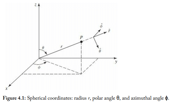
First of all we need to rewrite $L_x, L_y$, and $L_z$ in spherical coordinates. Now, $\mathbf{L}=-i \hbar(\mathbf{r} \times \nabla)$, and the gradient, in spherical coordinates, is: $\frac{.33}{}$
$$
\nabla=\hat{r} \frac{\partial}{\partial r}+\hat{\theta} \frac{1}{r} \frac{\partial}{\partial \theta}+\hat{\phi} \frac{1}{r \sin \theta} \frac{\partial}{\partial \phi}
$$
meanwhile, $\mathbf{r}=r \hat{r}$, so
$$
\begin{aligned}
\mathbf{L} & =-i \hbar\left[r(\hat{r} \times \hat{r}) \frac{\partial}{\partial r}+(\hat{r} \times \hat{\theta}) \frac{\partial}{\partial \theta}+(\hat{r} \times \hat{\phi}) \frac{1}{\sin \theta} \frac{\partial}{\partial \phi}\right] . \
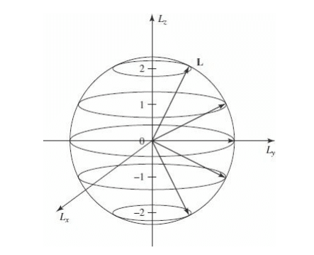
\operatorname{But}(\hat{r} \times \hat{r}) & =0,(\hat{r} \times \hat{\theta})=\hat{\phi}, \text { and }(\hat{r} \times \hat{\phi})=-\hat{\theta} \text { (see Figure 4.1), and hence } \
\mathbf{L} & =-i \hbar\left(\hat{\phi} \frac{\partial}{\partial \theta}-\hat{\theta} \frac{1}{\sin \theta} \frac{\partial}{\partial \phi}\right) .
\end{aligned}
$$
The unit vectors $\hat{\theta}$ and $\hat{\phi}$ can be resolved into their cartesian components:
$$
\begin{aligned}
& \hat{\theta}=(\cos \theta \cos \phi) \hat{\imath}+(\cos \theta \sin \phi) \hat{\jmath}-(\sin \theta) \hat{k} ; \
& \hat{\phi}=-(\sin \phi) \hat{\imath}+(\cos \phi) \hat{\jmath} .
\end{aligned}
$$
Thus
$$
\begin{aligned}
\mathbf{L} & =-i \hbar\left[(-\sin \phi \hat{\imath}+\cos \phi \hat{\jmath}) \frac{\partial}{\partial \theta}\right. \
& \left.-(\cos \theta \cos \phi \hat{\imath}+\cos \theta \sin \phi \hat{\jmath}-\sin \theta \hat{k}) \frac{1}{\sin \theta} \frac{\partial}{\partial \phi}\right] .
\end{aligned}
$$
量子力学代写
物理代写|量子力学代写Quantum mechanics代考|Eigenvalues
操作员$L_x$和$L_y$不通勤;事实上
$$
\begin{aligned}
{\left[L_x, L_y\right] } & =\left[y p_z-z p_y, z p_x-x p_z\right] \
& =\left[y p_z, z p_x\right]-\left[y p_z, x p_z\right]-\left[z p_y, z p_x\right]+\left[z p_y, x p_z\right] .
\end{aligned}
$$
从正则交换关系(公式4.10)我们知道,这里唯一不能交换的运算符是$x$与$p_x, y$与$p_y$,以及$z$与$p_z$。中间的两项去掉了,剩下
$$
\left[L_x, L_y\right]=y p_x\left[p_z, z\right]+x p_y\left[z, p_z\right]=i \hbar\left(x p_y-y p_x\right)=i \hbar L_z .
$$
当然,我们可以从$\left[L_y, L_z\right]$或$\left[L_z, L_x\right]$开始,但没有必要单独计算这些-我们可以通过索引$(x \rightarrow y, y \rightarrow z, z \rightarrow x)$的循环排列立即得到它们:
$$
\left[L_x, L_y\right]=i \hbar L_z ; \quad\left[L_y, L_z\right]=i \hbar L_x ; \quad\left[L_z, L_x\right]=i \hbar L_y
$$
这些是角动量的基本交换关系;一切都从它们开始。
注意$L_x, L_y$和$L_z$是不兼容的可观察对象。根据广义不确定性原理(式3.62),
$$
\sigma_{L_x}^2 \sigma_{L_y}^2 \geq\left(\frac{1}{2 i}\left\langle i \hbar L_z\right\rangle\right)^2=\frac{\hbar^2}{4}\left\langle L_z\right\rangle^2,
$$
或
$$
\sigma_{L_x} \sigma_{L_y} \geq \frac{\hbar}{2}\left|\left\langle L_z\right\rangle\right|
$$
因此,寻找同时是$L_x$和$L_y$的特征函数的状态是徒劳的另一方面,总角动量的平方,
$$
L^2 \equiv L_x^2+L_y^2+L_z^2
$$
是否与$L_x$通勤:
$$
\begin{aligned}
{\left[L^2, L_x\right] } & =\left[L_x^2, L_x\right]+\left[L_y^2, L_x\right]+\left[L_z^2, L_x\right] \
& =L_y\left[L_y, L_x\right]+\left[L_y, L_x\right] L_y+L_z\left[L_z, L_x\right]+\left[L_z, L_x\right] L_z \
& =L_y\left(-i \hbar L_z\right)+\left(-i \hbar L_z\right) L_y+L_z\left(i \hbar L_y\right)+\left(i \hbar L_y\right) L_z \
& =0 .
\end{aligned}
$$
物理代写|量子力学代写Quantum mechanics代考|Eigenfunctions
首先我们需要在球坐标下重写$L_x, L_y$和$L_z$。现在是$\mathbf{L}=-i \hbar(\mathbf{r} \times \nabla)$,在球坐标下,梯度是$\frac{.33}{}$
$$
\nabla=\hat{r} \frac{\partial}{\partial r}+\hat{\theta} \frac{1}{r} \frac{\partial}{\partial \theta}+\hat{\phi} \frac{1}{r \sin \theta} \frac{\partial}{\partial \phi}
$$
同时,$\mathbf{r}=r \hat{r}$
$$
\begin{aligned}
\mathbf{L} & =-i \hbar\left[r(\hat{r} \times \hat{r}) \frac{\partial}{\partial r}+(\hat{r} \times \hat{\theta}) \frac{\partial}{\partial \theta}+(\hat{r} \times \hat{\phi}) \frac{1}{\sin \theta} \frac{\partial}{\partial \phi}\right] . \
\operatorname{But}(\hat{r} \times \hat{r}) & =0,(\hat{r} \times \hat{\theta})=\hat{\phi}, \text { and }(\hat{r} \times \hat{\phi})=-\hat{\theta} \text { (see Figure 4.1), and hence } \
\mathbf{L} & =-i \hbar\left(\hat{\phi} \frac{\partial}{\partial \theta}-\hat{\theta} \frac{1}{\sin \theta} \frac{\partial}{\partial \phi}\right) .
\end{aligned}
$$
单位矢量$\hat{\theta}$和$\hat{\phi}$可以分解成它们的直角分量:
$$
\begin{aligned}
& \hat{\theta}=(\cos \theta \cos \phi) \hat{\imath}+(\cos \theta \sin \phi) \hat{\jmath}-(\sin \theta) \hat{k} ; \
& \hat{\phi}=-(\sin \phi) \hat{\imath}+(\cos \phi) \hat{\jmath} .
\end{aligned}
$$
因此
$$
\begin{aligned}
\mathbf{L} & =-i \hbar\left[(-\sin \phi \hat{\imath}+\cos \phi \hat{\jmath}) \frac{\partial}{\partial \theta}\right. \
& \left.-(\cos \theta \cos \phi \hat{\imath}+\cos \theta \sin \phi \hat{\jmath}-\sin \theta \hat{k}) \frac{1}{\sin \theta} \frac{\partial}{\partial \phi}\right] .
\end{aligned}
$$

物理代写|量子力学代写Quantum mechanics代考 请认准UprivateTA™. UprivateTA™为您的留学生涯保驾护航。
微观经济学代写
微观经济学是主流经济学的一个分支,研究个人和企业在做出有关稀缺资源分配的决策时的行为以及这些个人和企业之间的相互作用。my-assignmentexpert™ 为您的留学生涯保驾护航 在数学Mathematics作业代写方面已经树立了自己的口碑, 保证靠谱, 高质且原创的数学Mathematics代写服务。我们的专家在图论代写Graph Theory代写方面经验极为丰富,各种图论代写Graph Theory相关的作业也就用不着 说。
线性代数代写
线性代数是数学的一个分支,涉及线性方程,如:线性图,如:以及它们在向量空间和通过矩阵的表示。线性代数是几乎所有数学领域的核心。
博弈论代写
现代博弈论始于约翰-冯-诺伊曼(John von Neumann)提出的两人零和博弈中的混合策略均衡的观点及其证明。冯-诺依曼的原始证明使用了关于连续映射到紧凑凸集的布劳威尔定点定理,这成为博弈论和数学经济学的标准方法。在他的论文之后,1944年,他与奥斯卡-莫根斯特恩(Oskar Morgenstern)共同撰写了《游戏和经济行为理论》一书,该书考虑了几个参与者的合作游戏。这本书的第二版提供了预期效用的公理理论,使数理统计学家和经济学家能够处理不确定性下的决策。
微积分代写
微积分,最初被称为无穷小微积分或 “无穷小的微积分”,是对连续变化的数学研究,就像几何学是对形状的研究,而代数是对算术运算的概括研究一样。
它有两个主要分支,微分和积分;微分涉及瞬时变化率和曲线的斜率,而积分涉及数量的累积,以及曲线下或曲线之间的面积。这两个分支通过微积分的基本定理相互联系,它们利用了无限序列和无限级数收敛到一个明确定义的极限的基本概念 。
计量经济学代写
什么是计量经济学?
计量经济学是统计学和数学模型的定量应用,使用数据来发展理论或测试经济学中的现有假设,并根据历史数据预测未来趋势。它对现实世界的数据进行统计试验,然后将结果与被测试的理论进行比较和对比。
根据你是对测试现有理论感兴趣,还是对利用现有数据在这些观察的基础上提出新的假设感兴趣,计量经济学可以细分为两大类:理论和应用。那些经常从事这种实践的人通常被称为计量经济学家。
Matlab代写
MATLAB 是一种用于技术计算的高性能语言。它将计算、可视化和编程集成在一个易于使用的环境中,其中问题和解决方案以熟悉的数学符号表示。典型用途包括:数学和计算算法开发建模、仿真和原型制作数据分析、探索和可视化科学和工程图形应用程序开发,包括图形用户界面构建MATLAB 是一个交互式系统,其基本数据元素是一个不需要维度的数组。这使您可以解决许多技术计算问题,尤其是那些具有矩阵和向量公式的问题,而只需用 C 或 Fortran 等标量非交互式语言编写程序所需的时间的一小部分。MATLAB 名称代表矩阵实验室。MATLAB 最初的编写目的是提供对由 LINPACK 和 EISPACK 项目开发的矩阵软件的轻松访问,这两个项目共同代表了矩阵计算软件的最新技术。MATLAB 经过多年的发展,得到了许多用户的投入。在大学环境中,它是数学、工程和科学入门和高级课程的标准教学工具。在工业领域,MATLAB 是高效研究、开发和分析的首选工具。MATLAB 具有一系列称为工具箱的特定于应用程序的解决方案。对于大多数 MATLAB 用户来说非常重要,工具箱允许您学习和应用专业技术。工具箱是 MATLAB 函数(M 文件)的综合集合,可扩展 MATLAB 环境以解决特定类别的问题。可用工具箱的领域包括信号处理、控制系统、神经网络、模糊逻辑、小波、仿真等。