MY-ASSIGNMENTEXPERT™可以为您提供 my.uq.edu.au ECON2300 Econometrics计量经济学的代写代考和辅导服务!
这是昆士兰大学计量经济学课程的代写成功案例。
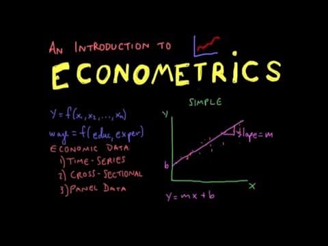
ECON2300课程简介
Course description
Introductory applied econometric course for students with basic economic statistics background. Topics covered include: economic models and role of econometrics, linear regression with single and multiple regressors, hypothesis testing and confidence intervals, dummy variables and nonlinear regression functions, internal and external validity of regression models, panel data models, binary response models, instrumental variable regressions, experiments and quasi-experiments, as well as basic time series analysis. Practical problems are solved using the R econometrics software.
Prerequisites
This is an introductory course in applied econometrics. It reviews and builds on the simple linear regression model taught in introductory statistics courses such as ECON1310 and ECON1320. The models studied in this course have numerous applications in economics, finance, marketing, management and related areas. A feature of the course is the way examples and exercises are drawn from these different discipline areas to illustrate the usefulness and limitations of certain econometric/statistical techniques. Hands-on experience in applying these techniques is gained through the use of R, an econometric computer software package available in the BEL computer laboratories.
ECON2300 Econometrics HELP(EXAM HELP, ONLINE TUTOR)
From Wool C5.3 Suppose you are interested in the effect of parental education on child birthweights.
a. Your initial model is $b w g h t=\beta_0+\beta_1$ motheduc $+u$
Suppose that mothereduc was a binary variable that was equal to 1 if a mother had completed high school and 0 if a mother had not completed high school. Interpret the coefficients $\beta_0$ and $\beta_1$. [I’m not asking you to run this regression, just explain how to interpret coefficients on binary variables.]
b. Your next model is $b w g h t=\beta_0+\beta_1$ cigs $+\beta_2$ parity $+\beta_3$ faminc $+\beta_4$ motheduc $+\beta_5$ fatheduc $+u$
Suppose that faminc was measured in logs. How would you interpret $\beta_3$ ? [I’m not asking you to run this regression, just explain how to interpret coefficients on logged variables.]
c. Your next model is $b w g h t=\beta_0+\beta_1$ cigs $+\beta_2$ parity $+\beta_3$ faminc $+\beta_4$ faminc $^2+\beta_5$ motheduc $+\beta_6$ fatheduc $+u$
How would you explain the effect of family income? I’m not asking you to run this regression, just explain how to interpret coefficients in quadratic models.
a. $\beta_0$ is the mean (average) birthweight for children whose mother’s did not complete high school. $\beta_1$ is the difference in mean (average) birthweights between children whose mothers’ did and di not complete high school.
b. If income is measured in logs, a $1 \%$ increase in income is associated with a $\beta_1$ increase in ounces of birthweight. For example, if $\widehat{\beta}_1=.3$, a $1 \%$ increase in income is associated with a 3 ounce increase in birthweight.
c. To interpret quadratic specifications, take a partial derivative. The effect of family income on birthweight $=\partial$ birthweight $/$ ofamily income $=\beta_3+\beta_4$ faminc. You will need to choose a level of family income to report a specific marginal effect. Often this is reported at the mean.
Show that the estimated coefficient $\widehat{\beta}_1$ and estimated standard errors for $\widehat{\beta}_1$ in this 2 variable regression model
(a) $\left(y_i\right)=\widehat{\beta}_0+\widehat{\beta}_1\left(x_i\right)+\hat{u}_i$
are equivalent to those in this model
(b) $\left(y_i-\bar{y}\right)=\widehat{\beta}_1\left(x_i-\bar{x}\right)+\hat{u}_i$
If you need to draw on other assumptions/properties of the QLS estimator in your derivation, state these.
Show that the estimated coefficient $\widehat{\beta}_1$ and estimated standard errors for $\widehat{\beta}_1$ in this 2 variable regression model
(a) $\left(y_i\right)=\widehat{\beta}_0+\widehat{\beta}_1\left(x_i\right)+\hat{u}_i$
are equivalent to those in this model,
(b) $\left(y_i-\bar{y}\right)=\hat{\beta}_1\left(x_i-\bar{x}\right)+\hat{u}_i$
If you need to draw on other assumptions/properties of the QLS estimator in your derivation, state these.
To show the coefficients are the same, use property that regression line runs through mean of data: $\widehat{\beta}_0=\bar{y}-\widehat{\beta}_1 \bar{x}$
This is derived in the handout showing the derivation of the QLS estimators $\hat{\beta}_0, \hat{\beta}_1$ from minimizing the sum of squared errors. (Review that handout if needed.)
Plug this in and simplify to get the second expression
To show that the standard errors are the same, recall that for the first regression model,
$$
\operatorname{se}\left(\widehat{\beta}_1\right)=\left[\frac{\left(\frac{1}{n-2} \sum \hat{u}_i^2\right)^{1 / 2}}{\left(\sum\left(x_i-\bar{x}\right)^2\right)^{1 / 2}}\right]
$$
For the numerator, note that the $\hat{u}_i$ will be the same in (a) and (b) (this is also true because the mean of the estimated errors is zero). Therefore the numerator of the standard errors for (a) and (b) will be the same.
To show that denominators in the standard errors are the same, show that
$$
\left.\sum\left(x_i-\bar{x}\right)^{2+}=\sum\left(\left(x_i-\bar{x}\right)-\overline{\left(x_i-\bar{x}\right.}\right)\right)^{2-}
$$
I’ll let you work through that algebra on your own.

MY-ASSIGNMENTEXPERT™可以为您提供 MY.UQ.EDU.AU EC309 ECONOMETRICS计量经济学的代写代考和辅导服务