经济代写|ECON2300 Econometrics

MY-ASSIGNMENTEXPERT™可以为您提供 my.uq.edu.au ECON2300 Econometrics计量经济学的代写代考和辅导服务！

这是昆士兰大学计量经济学课程的代写成功案例。

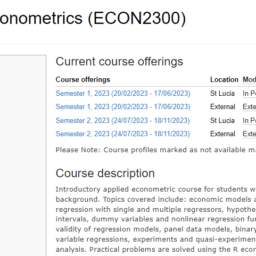
ECON2300课程简介

Course description

Introductory applied econometric course for students with basic economic statistics background. Topics covered include: economic models and role of econometrics, linear regression with single and multiple regressors, hypothesis testing and confidence intervals, dummy variables and nonlinear regression functions, internal and external validity of regression models, panel data models, binary response models, instrumental variable regressions, experiments and quasi-experiments, as well as basic time series analysis. Practical problems are solved using the R econometrics software.

Prerequisites 

This is an introductory course in applied econometrics. It reviews and builds on the simple linear regression model taught in introductory statistics courses such as ECON1310 and ECON1320. The models studied in this course have numerous applications in economics, finance, marketing, management and related areas. A feature of the course is the way examples and exercises are drawn from these different discipline areas to illustrate the usefulness and limitations of certain econometric/statistical techniques. Hands-on experience in applying these techniques is gained through the use of R, an econometric computer software package available in the BEL computer laboratories.

ECON2300 Econometrics HELP（EXAM HELP， ONLINE TUTOR）

From Wool 8.7Consider a model at the employee level.
$$
y_{i \xi}=\beta_o+\beta_{l+x_{i e, 1}}+\text { wes }+\beta_k x_{i e, k}+f_i+y_{i e}
$$
where the unobserved variable $f_i$ is a “firm effect” to each employee $e$ at a given firm $i$. The error term $v_{j e}$ is an individual specific error term-that is, it is specific to each individual at each firm. The composite error is $\mu_{i f}=f_i+y_{j e}$ (as in equation 8.28).
(a) Assume that $\operatorname{Var}\left(f_j\right)=\sigma_f^2$ and $\operatorname{Var}\left(v_{i \varepsilon}\right)=\sigma_v^2$ and $f_i$ and $v_{i j}$ are uncorrelated. Show that $\operatorname{Var}\left(u_{i \varepsilon}\right)=\sigma_f^2+\sigma_v^2$.
This follows from the simple fact that, for uncorrelated random variables, the variance of the sum is the sum of the variances: $\operatorname{Var}\left(f_i+v_{i, \varepsilon}\right)=\operatorname{Var}\left(f_i\right)+\operatorname{Var}\left(v_{i, \varepsilon}\right)=\sigma_f^2+\sigma_v^2$.
(b) Now suppose that for $\mathrm{e} \neq \mathrm{g}$ (that is, we are looking at two different employees), $v_{i g}$ and $y_{i g}$ are uncorrelated. Show that $\operatorname{Cov}\left(u_{i g} u_{i g}\right)=$
$$
\sigma_f^2 \text {. }
$$

We compute the covariance between any two of the composite errors as
$$
\begin{aligned}
\operatorname{Cov}\left(u_{i, s}, u_{i g}\right) & =\operatorname{Cov}\left(f_i+v_{i, s}, f_i+v_{i g}\right)=\operatorname{Cov}\left(f_i, f_i\right)+\operatorname{Cov}\left(f_i, v_{i g}\right)+\operatorname{Cov}\left(v_{i, s}, f_i\right)+\operatorname{Cov}\left(v_{i,}, v_{i g}\right) \
& =\operatorname{Var}\left(f_i\right)+0+0+0=\sigma_f^2,
\end{aligned}
$$
where we use the fact that the covariance of a random variable with itself is its variance and the assumptions that $f_{\mathrm{t}}, v_{\mathrm{t}, \varepsilon}$, and $v_{\mathrm{t}, g}$ are pairwise uncorrelated.
(c) Let –that is the average composite error within a firm
$$
\operatorname{var}\left(\bar{u}i\right)=\sigma_f^2+\frac{\sigma_v^2}{m_i} $$ with $m{\mathrm{i}}$ employees. Show that This is most easily solved by writing
$$
m_i^{-1} \sum_{:=1}^{m_i} u_{i, \varepsilon}=m_i^{-1} \sum_{:-1}^{m_i}\left(f_i+u_{i, \varepsilon}\right)=f_i+m_i^{-1} \sum_{s=1}^{m_i} v_{i, \varepsilon} .
$$

Now, by assumption, $f_i$ is uncorrelated with each term in the last sum; therefore, $f_i$ is uncorrelated with It follows that
$$
\begin{aligned}
\operatorname{Var}\left(f_i+m_i^{-1} \sum_{i=1}^m v_{i, \varepsilon}\right) & =\operatorname{Var}\left(f_i\right)+\operatorname{Var}\left(m_i^{-1} \sum_{i=1}^m v_{i, \varepsilon}\right) \
& =\sigma_f^2+\sigma_v^2 / m_i,
\end{aligned}
$$
where we use the fact that the variance of an average of $m_i$ uncorrelated random variables with common variance $\sigma_v^{\sigma_v^2}$ in this case) is simply the common variance divided by $m_i$ – the usual formula for a sample average from a random sample.
(d) Discuss the relevance of part (iii) for WLS estimation using data averaged at the firm level, where the weight used for observation $i$ is the usual firm size.
The standard weighting ignores the variance of the firm effect, $\sigma_t^2$, Thus, the (incorrect) weight function used is ${ }^{1 / h_{\mathrm{i}}=m_{\mathrm{i}}}$. A valid weighting function is obtained by writing the variance from (iii) as $\operatorname{Var}\left(\bar{u}_i\right)=\sigma_f^2\left[1+\left(\sigma_v^2 / \sigma_f^2\right) / m_i\right]=\sigma_f^2 h_i$. But obtaining the proper weights requires us to know (or be able to estimate) the ratio $\sigma_v^2 / \sigma_f^2$. Estimation is possible, but we do not discuss that here. In any event, the usual weight is incorrect. When the mire large or, the ratio $\sigma_v^2 / \sigma_f^2$ is small – so that the firm effect is more important than the individual-specific effect-the correct weights are close to being constant. Thus, attaching large weights to large firms may be quite inappropriate.

MY-ASSIGNMENTEXPERT™可以为您提供 MY.UQ.EDU.AU EC309 ECONOMETRICS计量经济学的代写代考和辅导服务