MY-ASSIGNMENTEXPERT™可以为您提供 my.uq.edu.au ECON2300 Econometrics计量经济学的代写代考和辅导服务!
这是昆士兰大学计量经济学课程的代写成功案例。
ECON2300课程简介
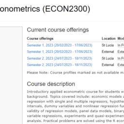
Course description
Introductory applied econometric course for students with basic economic statistics background. Topics covered include: economic models and role of econometrics, linear regression with single and multiple regressors, hypothesis testing and confidence intervals, dummy variables and nonlinear regression functions, internal and external validity of regression models, panel data models, binary response models, instrumental variable regressions, experiments and quasi-experiments, as well as basic time series analysis. Practical problems are solved using the R econometrics software.
Prerequisites
This is an introductory course in applied econometrics. It reviews and builds on the simple linear regression model taught in introductory statistics courses such as ECON1310 and ECON1320. The models studied in this course have numerous applications in economics, finance, marketing, management and related areas. A feature of the course is the way examples and exercises are drawn from these different discipline areas to illustrate the usefulness and limitations of certain econometric/statistical techniques. Hands-on experience in applying these techniques is gained through the use of R, an econometric computer software package available in the BEL computer laboratories.
ECON2300 Econometrics HELP(EXAM HELP, ONLINE TUTOR)
Show that the estimated coefficient $\widehat{\beta}_1$ and estimated standard errors for $\widehat{\beta}_1$ in this 2 variable regression model
(a) $\left(y_i\right)=\widehat{\beta}_0+\widehat{\beta}_1\left(x_i\right)+\hat{u}_i$
are equivalent to those in this model
(b) $\left(y_i-\bar{y}\right)=\hat{\beta}_1\left(x_i-\bar{x}\right)+\hat{u}_i$
If you need to draw on other assumptions/properties of the QLS estimator in your derivation, state these.
Show that the estimated coefficient $\widehat{\beta}_1$ and estimated standard errors for $\widehat{\beta}_1$ in this 2 variable regression model
(a) $\left(y_i\right)=\hat{\beta}_0+\hat{\beta}_1\left(x_i\right)+\hat{u}_i$
are equivalent to those in this model
(b) $\left(y_i-\bar{y}\right)=\hat{\beta}_1\left(x_i-\bar{x}\right)+\hat{u}_i$
If you need to draw on other assumptions/properties of the QLS estimator in your derivation, state these.
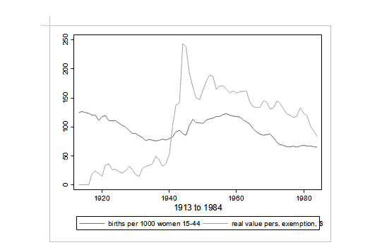
(Adapted from C11.5, C12.1) Suppose we are interested in how personal tax exemptions (pe) affect the general fertility rate (gfr). Use the data in FERTIL 3.RAW for this exercise.
i. Estimate the following equation:
$$
g f_{\mathrm{t}}=\beta_0+\beta_1 p_{e_t}+\beta_2 w w 2_{\mathrm{t}}+\beta_3 p i l_{\mathrm{t}}+\varepsilon_{\mathrm{t}}
$$
where $w w 2$ is a dummy variable for the years 1941-1945, and pill is a dummy variable that is equal to one for the years 1963 on (after the pill was available). Discuss the significance of the coefficients and interpret their magnitudes.
ii. Fertility may react to personal exemptions with a lag. Reestimate your equation adding 2 lags of $p e$ (pet-j and pet-2). Are these variables jointly significant? What are the degrees of freedom of your F-test and why?
iii. What are the first order autecorrelations ( $\hat{\rho}_1$ ) for $g f x$ and $p e$ ? What do these suggest about possible unit root(s)? What does this suggest about your OLS results in (i)?
iv. Re-estimate (i) using first differences-that is, changes in gf and changes in pe. (Do not difference $w w 2$ and pill.) How does the effect of pe compare with your estimates in levels in (i)?
v. Reestimate (ii) using first differences of gft, pe, and lagged pe. (Again, do not difference $w w 2$ and pill.) Interpret the coefficients and comment on their statistical significance.
vi. Add a linear time trend to the model in (v). Is a time trend necessary in the firstdifference equation?
vii. Using the model in (vi), test for whether there is AR(1) serial correlation in the errors.
Suppose we are interested in how laws and economic conditions might affect driving behavior. Use TRAFFIC2.RAW (monthly observations from CA from Jan 1981-Dec 1989) to answer these questions.
a. The variable prcfat is the percentage of accidents resulting in at least on fatality. Note that this variable is a percentage, not a proportion. What is the average of this variable over this period?
b. Run a regression of prcfat on a linear time trend, 11 monthly dummies (set January as your base month), wkends, ynem, spdlaw, and beltlaw. Discuss the estimated effects of unem, spdlaw, and beltlaw. Do the signs and magnitudes make sense to you?
c. Test the errors for AR(1) serial correlation.
d. Re-estimate the model accounting to serial correlation.
e. Compute the first order autocorrelations $\left(\hat{\rho}_1\right.$ ) for ynem and prcfat. What do these suggest about possible unit root(s)?
f. Estimate the model in (ii) using first differences for unem and prcfat (Do not difference the month or policy variables.) Compare your results to those in (ii).
Use the data in PHIIPSRAW for this exercise. (This follows several of the examples in Wooldridge, but using the full set of the data, rather than only through 1996.)
The Phillips curve posits a relationship between unemployment and inflation:
$$
\inf f_t-\inf f_t^e=\beta_1\left(\text { unem }t-\mu_0\right)+e_t $$ Here inf $f_t$ is the expected rate of inflation for year $t$ that was formed in year $t-1$. The above formulation posits that there is a relationship between unanticipated inflation (deviations from expectations) and cyclical unemployment-deviations of unemployment in year $\mathrm{t}$ from the natural rate of unemployment, $\mu{0,}$ One assumption of this model is that the natural rate of unemployment is constant.
Under the adaptive expectations model, current expected values of inflation depend on recently observed inflation, resulting in the following:
$$
\begin{aligned}
& \inf t-\inf f{t-1}=\beta_0+\beta_1\left(\text { unem }_t\right)+e_t=\Delta \inf _t=\beta_0+\beta_1\left(\text { unem }_t\right)+e_t \
& \text { where } \beta_0=-\beta_1 \mu_0
\end{aligned}
$$
a. Estimate the effect of unemployment on the levels of inflation (rather than the change in inflation). Interpret the coefficients. Using your estimates, calculate the natural rate of unemployment.
b. Obtain the residuals from this estimation. Is there evidence of serial correlation in these residuals?
c. Re-estimate this model accounting for serial correlation using the Prais-Winsten method of FGLS. Comment on the difference in coefficient estimates.
d. Then estimate the adaptive expectations model: $\Delta$ inf $f_t=\beta_0+\beta_1\left(\right.$ unem $\left._t\right)+e_t$ Obtain the residuals from this estimation? Is there evidence of serial correlation in these residuals? If there is, re-estimate the model.
e. An alternative model (the expectations augmented Phillips curve) allows the natural rate of unemployment to depend on past levels of unemployment. Reestimate the above model using changes in unemployment rather than levels as the independent variable. Comment on the difference between your results here and those in (a).
f. Compute a first order autocorrelation for unem. Is the root close to one? (Not asking for a formal test here.)
g. Based on what you found from your various estimation results using different models and on the autocorrelations in errors and in the series, explain the pattern of your results. What would you conclude about which model is most appropriate?

MY-ASSIGNMENTEXPERT™可以为您提供 MY.UQ.EDU.AU EC309 ECONOMETRICS计量经济学的代写代考和辅导服务