MY-ASSIGNMENTEXPERT™可以为您提供 my.uq.edu.au ECON2300 Econometrics计量经济学的代写代考和辅导服务!
这是昆士兰大学计量经济学课程的代写成功案例。
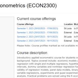
ECON2300课程简介
Course description
Introductory applied econometric course for students with basic economic statistics background. Topics covered include: economic models and role of econometrics, linear regression with single and multiple regressors, hypothesis testing and confidence intervals, dummy variables and nonlinear regression functions, internal and external validity of regression models, panel data models, binary response models, instrumental variable regressions, experiments and quasi-experiments, as well as basic time series analysis. Practical problems are solved using the R econometrics software.
Prerequisites
This is an introductory course in applied econometrics. It reviews and builds on the simple linear regression model taught in introductory statistics courses such as ECON1310 and ECON1320. The models studied in this course have numerous applications in economics, finance, marketing, management and related areas. A feature of the course is the way examples and exercises are drawn from these different discipline areas to illustrate the usefulness and limitations of certain econometric/statistical techniques. Hands-on experience in applying these techniques is gained through the use of R, an econometric computer software package available in the BEL computer laboratories.
ECON2300 Econometrics HELP(EXAM HELP, ONLINE TUTOR)
(From 13.6) In 1985, neither Florida nor Georgia had laws banning open alcohol containers in vehicle compartments. By 1990, Florida had passed such a law, but Georgia had not.
a. Suppose you can collect random samples of the driving age population in both states, for 1985 and 1990. Let arrest be a binary variable equal to unity if a person was arrested for drunk driving during the year. Without controlling for any factors, write down a linear probability model that allows you to test whether the open container law reduced the probability of being arrested for drunk driving. Which coefficient in your model measures the effect of the law?
Let FL be a binary variable equal to one if a person lives in Florida, and zero otherwise. Let 900 be a year dummy variable for 1990. Then we have the linear probability model
$$
\text { arrest }=\beta_0+\delta_0 y 90+\beta_1 F L+\delta_1 y 90 \cdot F L+u .
$$
The effect of the law is measured by $\delta_1$, which is the change in the probability of drunk driving arrest due to the new law in Florida. Including y90 allows for aggregate trends in drunk driving arrests that would affect both states; including FL allows for systematic differences between Florida and Georgia in either drunk driving behavior or law enforcement
Why might you want to control for other factors in the model? What other factors might you want to include?
Any factor that leads to different overall trends in both states could be relevant. I am not concerned to include things that are different across the states but are constant over time -the Florida dummy will account for these. But it could be that the populations of drivers in the two states change in different ways over time. For example, age, race, or gender distributions may have changed. The levels of education across the two states may have changed. As these factors might affect whether someone is arrested for drunk driving, it could be important to control for them. At a minimum, there is the possibility of obtaining a more precise estimator of $\delta_1$ by reducing the error variance. Essentially, any explanatory variable that affects arrest can be used for this purpose.
Now, suppose you can only collect data for 1985 and 1990 and the county level for the two states. The dependent variable would be the fraction of licensed drivers arrested for drunk driving during the year. How does the data structure differ from the individual level data described in part (a)? What econometric method would you use?
With this set up, I now have actual arrest rates, instead of only a sample, reducing the error from sampling. The interpretation of the coefficients will differ, because they represent averages across counties in a given state rather than state level averages. (Weighting by population is one option to deal with this). However, individual level dta allows me to control for individual level variation more effectively, which potentially may reduce my standard errors. I could also use a first difference, because I have the same set of counties in both years observed at two points in time.
See discussion in class. There are a number of different potential ways to approach this – are we trying to estimate the effect of attending a tribal college on an individual’s health relative to not attending college at all? Relative to attending a non-tribal college? Relative to the average of what individuals typically do if they do not attend a tribal college? Or are we interested in the effect of a tribal college on an entire community’s health? Would we expect spillovers to non-native populations?
For example, consider a triple difference with two years of data (PRE and POST):
Compare natives and non natives in counties with tribal colleges in the years after the tribal college was established
Relative to that same comparison in years before the tribal college was established
And then compare that to areas without tribal colleges:
(AMINDpost-AMINDpre)college counties – (NQNpost – NQNpre)college counties
(AMINDpost – AMIDpre)non college counties – (NQNpost – NQNpre)non college counties
That tells you that your equation needs at least 8 terms (including the constant) to pick up each of those averages. It’s easiest to start writing this by looking at the last terms of my difference (Non/pre/non-college) and working backwards:
$$
\begin{aligned}
& Y i, c, t=\beta 0+\beta 1 \text { POSTt }+\beta 2 \text { AMINDic, }, t+\beta 3 \text { AMINDi },, t{ }^* \text { POSTt+ } \beta 4 \text { TRIBAL },, t+ \
& \beta 5 \text { TRIBAL }, . t^* \text { POSTt + } \beta 6 \text { TRIBAL }, t^* \text { AMINDi.c, }+ \
& \text { B7TRIBAL }, t^* \text { AMINDi }, \text {, t*POSTt + eict } \
&
\end{aligned}
$$
$\mathrm{Y}$ is the health outcome of interest, AMIND is a dummy variable for whether an individual is Native American, TRIBAL is a dummy variable for a county that has a tribal college in existence, and POST is the second period.
If you had multiple years and multiple counties and enough data for lots of individuals within a county (both American Indians and non-American Indians), you could include year fixed effects (instead of the separate POST term) and county fixed effects (instead of the separate TRIBAL term).

MY-ASSIGNMENTEXPERT™可以为您提供 MY.UQ.EDU.AU EC309 ECONOMETRICS计量经济学的代写代考和辅导服务