MY-ASSIGNMENTEXPERT™可以为您提供sydney MATH1013 Mathematical Modeling数学建模的代写代考和辅导服务!
这是悉尼大学数学建模课程的代写成功案例。

MATH1013课程简介
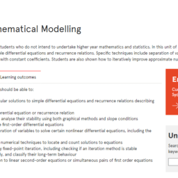
MATH1013 is designed for science students who do not intend to undertake higher year mathematics and statistics. In this unit of study students learn how to construct, interpret and solve simple differential equations and recurrence relations. Specific techniques include separation of variables, partial fractions and first and second order linear equations with constant coefficients. Students are also shown how to iteratively improve approximate numerical solutions to equations.
Prerequisites
At the completion of this unit, you should be able to:
- LO1. write down general and particular solutions to simple differential equations and recurrence relations describing models of growth and decay
- LO2. determine the order of a differential equation or recurrence relation
- LO3. find equilibrium solutions and analyse their stability using both graphical methods and slope conditions
- LO4. recognise and solve separable first-order differential equations
- LO5. use partial fractions and separation of variables to solve certain nonlinear differential equations, including the logistic equation
- LO6. use a variety of graphical and numerical techniques to locate and count solutions to equations
- LO7. solve equations numerically by fixed-point iteration, including checking if an iteration method is stable
- LO8. explore sequences numerically, and classify their long-term behaviour
- LO9. determine the general solution to linear second-order equations or simultaneous pairs of first order equations with constant coefficients.
MATH1013 Mathematical Modeling HELP(EXAM HELP, ONLINE TUTOR)
a. During the ‘free-fall’ portion of her descent, a sky-diver of mass $m=75 \mathrm{~kg}$ (including equipment) has terminal speed $\left|v_T\right|=50 \mathrm{~m} \mathrm{~s}^{-1}$. Assuming positive displacement downward, an appropriate IVP is
$$
m \frac{d v}{d t}=m g-\beta v^2, v(0)=0
$$
State the role of each term, find the dimensions of the positive constant $\beta$, and estimate its numerical value. (Use $g=10 \mathrm{~m} \mathrm{~s}^{-2}$.)
b. For any positive values of $m, g$, and $\beta$, show that $u=\frac{v}{a}$ and $\tau=\frac{t}{a / g}$ are dimensionless variables, where $a=\sqrt{\frac{m g}{\beta}}$. Hence derive the equivalent dimensionless IVP
$$
\frac{d u}{d \tau}=1-u^2, u(0)=0, \text { for } 0 \leq u \leq 1
$$
c. Solve the DE in part b. using partial fractions. Hence find the solution of the IVP in part a., and confirm that
$$
\lim _{t \rightarrow \infty}|v(t)|=50 \mathrm{~m} \mathrm{~s}^{-1}
$$
i.e., the terminal speed is the limit of $|v(t)|$ as $t \rightarrow \infty$.
d. Once the parachute opens, clearly the drag coefficient will change. Suppose that this happens at $t=10 \mathrm{~s}$, and the new DE for her velocity during the second stage of her descent is
$$
m \frac{d v}{d t}=m g-\gamma v^2
$$
Find a value for the positive constant $\gamma$ such that her new terminal velocity is $5 \mathrm{~m} \mathrm{~s}^{-1}$, a safe landing speed.
e. Will the transition be smooth? (Think about how the drag force will change at $t=10 \mathrm{~s}$.) What might help smooth this ‘jerk’?
A rubber balloon filled with helium rises vertically after being released from rest. Three forces act on the balloon: gravity, a resistive drag force proportional to the square of its speed, and the buoyant force due to the fact that helium is much less dense than air. Here are the relevant data.
The empty balloon has a mass of $10 \mathrm{~g}$.
The balloon filled with helium has volume $0.01 \mathrm{~m}^3$.
The density of helium is $0.2 \mathrm{~kg} \mathrm{~m}^{-3}$.
The density of air is $1.3 \mathrm{~kg} \mathrm{~m}^{-3}$.
Gravitational acceleration is $9.8 \mathrm{~m} \mathrm{~s}^{-2}$.
The constant of proportionality for the drag force is $\gamma=0.25 \mathrm{~N} \mathrm{~s}^2 \mathrm{~m}^{-2}$.
a. Formulate an IVP for the velocity $v(t)$ of the balloon, assuming displacement positive upward from the point of release at time $t=0$. DO NOT SOLVE.
b. Determine the terminal velocity of the balloon as it rises, if one exists.
c. Suppose a pinhole leak develops at some time $t_1>0$, when the velocity is $v_1$. The leak allows $1 \mathrm{~cm}^3 \mathrm{~s}^{-1}$ of the helium to escape, with velocity $u=v-0.002 \mathrm{~m} \mathrm{~s}^{-1}$.
i. Justify a new model for $v(t)$ given by
$$
m \frac{d v}{d t}+0.002 \frac{d m}{d t}=-m g-\beta v^2+B(t),
$$
where $B(t)$ is the (now variable) buoyant force, and $\beta=0.01 \mathrm{~N} \mathrm{~s}^2 \mathrm{~m}^{-2}$ is the new drag coefficient for the deflated balloon. (Use the general variable mass model of Module 2.)
ii. Find the volume $V(t)$, the mass $m(t)$, and the buoyant force $B(t)$ under these circumstances, and determine the time $t^{\star}$ when the balloon is emptied of helium.
iii. WITHOUT CONSULTING ANY DEs, describe in your own words the motion of the balloon on three intervals:
- $0 \leq t \leq t_1$
- $t_1 \leq t \leq t^{\star}$
- $t>t^{\star}$
iv. Will the balloon have a terminal velocity in the interval $t>t^{\star}$ ? If so, what will it be?
Read carefully through the preamble on page 89 of your text (page 93 of Edition 1 , 91 of Edition 3), and problem 20 (6 in Edition 3) just below. Don’t solve problem 6 , as it is just logistic growth (with $r=\alpha$ and $K=1$ ), which we have studied in detail. However, do note the conclusion of this simple epidemic model, namely that eventually everyone becomes infectious.
Suppose local health care providers are able to isolate a fraction $\beta y$ of the infectious individuals per unit time, giving a new IVP
$$
\frac{d y}{d t}=\alpha y(1-y)-\beta y, \quad y(0)=y_0
$$
a. Show that, if $\alpha>\beta$, this model is equivalent to logistic growth (find the new $r$ and $K$ ), but that now not everyone eventually becomes infectious. DO NOT SOLVE the DE; use your prior knowledge of logistic growth and illustrate with two sketches, one showing a typical solution and any equilibria for $\beta=0$, the other for $0<\beta<\alpha$,
b. Show that, if $\alpha \leq \beta$, the epidemic dies out eventually. (Just examine the sign of $\frac{d y}{d t}$.) Illustrate your conclusions with two sketches of typical solutions and any equilibria, one for $\alpha=\beta$, and one for $\alpha<\beta$.
c. Explain why your answers to parts a. and b. make sense in terms of the roles of the parameters $\alpha$ and $\beta$ as they affect the growth and removal of infectives.
a. A population $p(t)$ of mice in a barn grows exponentially with intrinsic growth rate $r=0.1$ days $^{-1}$, but is ‘harvested’ by the resident tomcat at a constant rate of $h>0$ mice per day.
i. Justify the IVP $\frac{d p}{d t}=0.1 p-h, p(0)=p_0$ for this situation, explaining the role of each term.
ii. Using a qualitative analysis based on the signs of $\frac{d p}{d t}$ and $\frac{d^2 p}{d t^2}$, sketch typical solutions (including any equilibrium solutions), and sketch the phase line.
iii. Hence show that if $h \leq 0.1 p_0$, the mice survive, but if $h>0.1 p_0$, they are exterminated.
b. Suppose the barn’s resources are limited and will support at most $K$ mice, giving a revised model $\frac{d p}{d t}=0.1 p\left(1-\frac{p}{K}\right)-h, \quad p(0)=p_0$.
i. If $h=0$ (no tomcat), what type of growth results? Illustrate your answer with a sketch of typical solutions, for $p_0=\frac{3}{2} K, K, \frac{1}{2} K$, and $\frac{1}{10} K$. Show clearly any equilibrium solutions and their stability, and any changes in concavity.
ii. Suppose $K=200$ mice. Show that the model can be rewritten as
$$
\frac{d p}{d t}=f(p)=-0.0005\left((p-100)^2+2000(h-5)\right), \quad p(0)=p_0
$$
Hence explain why, if the tomcat kills more than 5 mice per day, the mice will be exterminated regardless of the value of $p_0$.
HINT: Examine the sign of $\frac{d p}{d t}$.
iii. What if the tomcat is not quite so deadly, and only kills 15 mice every 4 days (i.e., $h=3.75$ mice per day)? Show that in this case, the model can be rewritten as $\frac{d p}{d t}=f(p)=-0.0005(p-50)(p-150), \quad p(0)=p_0 \cdot($ ctd)
Sketch the graph of $f(p)$ for $p \geq 0$, and use qualitative analysis to sketch typical solutons for $p_0=40,50,75,100,150,175$. Sketch the phase line, and give the stability of any equilibria. State a sufficient condition on $p_0$ for the mice to survive in this case.

MY-ASSIGNMENTEXPERT™可以为您提供SYDNEY MATH1013 MATHEMATICAL MODELING数学建模的代写代考和辅导服务!