MY-ASSIGNMENTEXPERT™可以为您提供sydney MATH1013 Mathematical Modeling数学建模的代写代考和辅导服务!
这是悉尼大学数学建模课程的代写成功案例。
MATH1013课程简介
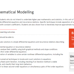
MATH1013 is designed for science students who do not intend to undertake higher year mathematics and statistics. In this unit of study students learn how to construct, interpret and solve simple differential equations and recurrence relations. Specific techniques include separation of variables, partial fractions and first and second order linear equations with constant coefficients. Students are also shown how to iteratively improve approximate numerical solutions to equations.
Prerequisites
At the completion of this unit, you should be able to:
- LO1. write down general and particular solutions to simple differential equations and recurrence relations describing models of growth and decay
- LO2. determine the order of a differential equation or recurrence relation
- LO3. find equilibrium solutions and analyse their stability using both graphical methods and slope conditions
- LO4. recognise and solve separable first-order differential equations
- LO5. use partial fractions and separation of variables to solve certain nonlinear differential equations, including the logistic equation
- LO6. use a variety of graphical and numerical techniques to locate and count solutions to equations
- LO7. solve equations numerically by fixed-point iteration, including checking if an iteration method is stable
- LO8. explore sequences numerically, and classify their long-term behaviour
- LO9. determine the general solution to linear second-order equations or simultaneous pairs of first order equations with constant coefficients.
MATH1013 Mathematical Modeling HELP(EXAM HELP, ONLINE TUTOR)
. Consider the system $\mathbf{x}^{\prime}=\mathbf{A} \mathbf{x}$ for each matrix (i) $\mathbf{A}=\left(\begin{array}{cc}6 & -3 \ 2 & 1\end{array}\right)$, (ii) $\mathbf{B}=\left(\begin{array}{cc}1 & 1 \ 5 & -3\end{array}\right)$.
a. Find the eigenvalues, eigenvectors (if any), and state the general solution.
b. Identify the type and stability of the equilibrium $\mathbf{x}=\mathbf{0}$ in each case.
c. Make a hand-drawn sketch of the phase portrait for each system by following the steps below and labelling your diagrams carefully.
- Find the nullclines and sketch them as dashed lines in the plane. Analyze the signs of $\frac{d x}{d t}$ and $\frac{d y}{d t}$ in each of the four regions between the nullclines, and show the orbit direction by an arrow on your sketch.
- Add the eigenvector directions (if any) to your sketch, in blue if they are stable solutions or red if unstable.
- Now that you have a framework for your phase portrait, and you have a good idea of the direction field, try to sketch several typical solutions. Verify your samples by doing a phase portrait in Maple if you like, but submit only hand drawn orbits for this question.
d. Find the equivalent second order DE for each system.
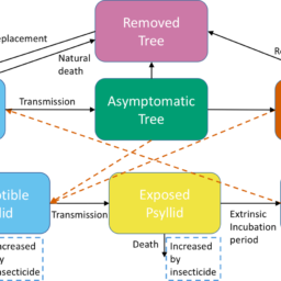
Tracers which can be detected by x-rays are often used to detect flow patterns in the body. One such tracer is inulin, which is injected into the blood, transfers back and forth between the bloodstream and intercellular areas, and also moves from the bloodstream into the urinary system.
Consider a compartment model for this process, as depicted in the diagram, where $X$ and $Y$ are the amounts of inulin in the bloodstream and the intercellular areas, respectively, and the positive constants $\mathrm{k}_i$ measure the proportions leaving/entering each compartment.
Thus the appropriate linear system if
$$
\frac{d}{d t} X(t)=-k_1 X-k_3 X+k_2 Y+I, \frac{d}{d t} Y(t)=k_1 X-k_2 Y
$$
where $I$ is the rate at which inulin is injected into the bloodstream.
a. Find the equilibrium point $\left(X_e, Y_e\right)$ of this system.
b. Translate the system, moving the equilibrium to the origin (as in Example 6.2.1), and find the eigenvalues of the translated system $\mathbf{x}^{\prime}=\mathbf{A x}$, where $\mathbf{x}(t)=(x(t), y(t))^T$, with $x(t)=X(t)-X_e$ and $y(t)=Y(t)-Y_e$.
c. Show that the equilibrium $\mathbf{x}(\mathbf{0})$ of the translated system is always an asymptotically stable node.
[HINT: If you let $s=k_1+k_2+k_3$, the discriminant in your solution for the eigenvalues should be $s^2-4 k_2 k_3$. Clearly this is less than $s^2$, but you will have to prove that it is always positive.]
d. Verify your result in c. for the values $k_1=0.01, k_2=0.02, k_3=0.005$, all measured in hour ${ }^{-1}$. If $I=1$ gram per hour, find the equilibrium levels of inulin in each compartment for these values.
e. Sketch the phase portrait of the original system for $(X(t), Y(t))$ for the values of the constants given in d.
Suggestion: Do this by using Maple to sketch the phase portrait of the translated system on $-1 \leq x \leq 1$ and $-1 \leq y \leq 1$. Then just make a hand-drawn sketch for the portrait of $(X, Y)$ with the equilibrium shifted to $\left(X_e, Y_e\right)$.
Eukaryotic cells are composed of several membrane-bound compartments. Certain molecules (e.g., oxygen) diffuse across these membranes according to Fick’s law, which states that the rate of flow is proportional to the difference in concentration, with the flow being from the compartment with the higher concentration to the one with lower concentration of that molecule.
Consider the simple case of two adjacent compartments of constant volumes $V_1$ and $V_2$, where molecules of a certain type diffuse freely across the separating membrane. Let $x$ and $y$ be the concentrations (i.e., mass per unit volume) of this species in the two compartments; thus the total masses are $x V_1$ and $y V_2$ respectively.
Then Fick’s law implies the system
$$
\begin{gathered}
\frac{d}{d t}\left(V_1 x(t)\right)=D(y(t)-x(t)), \frac{d}{d t}\left(V_2 y(t)\right)=D(x(t)-y(t)), \
\text { or } \quad \frac{d x}{d t}=\frac{D}{V_1}(y-x)=k_1(y-x), \frac{d y}{d t}=\frac{D}{V_2}(x-y)=k_2(x-y),
\end{gathered}
$$
where $D$ is a positive constant which quantifies how easily the molecules diffuse across the membrane, $k_1=\frac{D}{V_1}$, and $k_2=\frac{D}{V_2}$.
a. Explain how the terms in the model (initial version) are implied by Fick’s law.
b. Recalling that $\frac{d y}{d x}=\frac{\dot{y}}{\dot{x}}$, find an implicit equation for the orbits of this system, and show that this solution is simply a statement of conservation of total mass in the two compartments.
c. Write the system in the form $\dot{\mathbf{x}}=\mathbf{A} \mathbf{x}$, where $\mathbf{x}(t)=(x(t), y(t))^T$. Find the eigenvalues and eigenvectors of $\mathbf{A}$ and hence the general solution.
d. Describe the longterm behaviour of this system (i.e., what happens as $t \rightarrow \infty$ ) for any initial condition $\mathbf{x}(0)=\left(x_0, y_0\right)^T$, and give a physical interpretation.
e. Sketch the phase portrait in the positive quadrant for each of the three cases (i) $V_1V_2$. [HINT: Find the equilibria first.]
Before beginning this problem, review Exercise 6.2.2 in your lectures, which guides you through the derivation of the implicit and explicit solutions of the model for the simple pendulum with no damping. If you have not yet completed the exercise, it would be very helpful if you did so now.
Consider the linear system $\mathbf{x}^{\prime}(t)=\mathbf{A} \mathbf{x}=\left(\begin{array}{ll}-2 & \frac{5}{2} \ -2 & 2\end{array}\right) \mathbf{x}$, where $\mathbf{x}=\left(\begin{array}{l}x \ y\end{array}\right)$.
a. Show that the eigenvalues of this system imply a stable center.
b. Show that the system is equivalent to an implicit equation for the orbits,
$$
\frac{d y}{d x}=\frac{-4 x+4 y}{-4 x+5 y} .
$$
c. Write the DE in part b. in the form $M(x, y)+N(x, y) y^{\prime}=0$, and prove that it is exact. Then solve for the family of integral curves. (These curves must contain the orbits of the given linear system.)
d. The equation $\frac{(a x-b y)^2}{A^2}+\frac{(c x-f y)^2}{B^2}=1$ represents a ’tilted’ ellipse. By completing the square, show that the integral curves in part c. form a family of such ellipses. (This calculation is easier if you start with your integral curves in the form $x^2+\ldots=C$.) Plot three typical integral curves, $C=1,4,9$, using Maple’s implicitplot command (or otherwise). (A window $x=-7 . .7, y=-7 . .7$ works well for these values.) Then use the original system to determine the orbit nullclines, and the direction of the orbits, and add this information to your plot.
e. Find the equation of the particular integral curve through $(2,0)$. Show that, while the explicit functions $x(t)=4 \cos \omega t+2 \sin \omega t$, and $y(t)=4 \cos \omega t$ satisfy this equation for any constant $\omega$, they do not satisfy the given system $\mathbf{x}^{\prime}(t)=\mathbf{A} \mathbf{x}=\left(\begin{array}{ll}-2 & \frac{5}{2} \ -2 & 2\end{array}\right) \mathbf{x}$ unless $\omega=1$.
(This tells you that the DEs in the system impose a constraint on the period of the orbit which is not present in the implicit equation.)
It is true in general that the orbits of a stable center are ellipses.

MY-ASSIGNMENTEXPERT™可以为您提供SYDNEY MATH1013 MATHEMATICAL MODELING数学建模的代写代考和辅导服务!