MY-ASSIGNMENTEXPERT™可以为您提供sydney MATH1013 Mathematical Modeling数学建模的代写代考和辅导服务!
这是悉尼大学数学建模课程的代写成功案例。
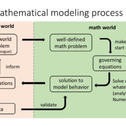
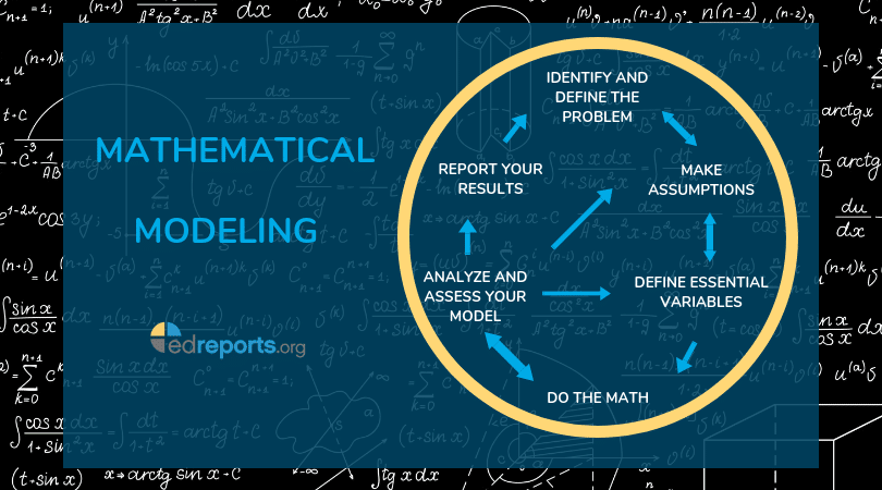
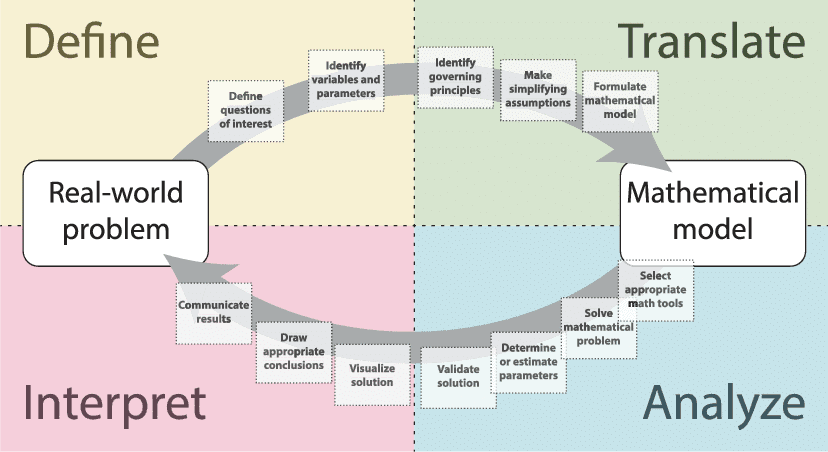
MATH1013课程简介
MATH1013 is designed for science students who do not intend to undertake higher year mathematics and statistics. In this unit of study students learn how to construct, interpret and solve simple differential equations and recurrence relations. Specific techniques include separation of variables, partial fractions and first and second order linear equations with constant coefficients. Students are also shown how to iteratively improve approximate numerical solutions to equations.
Prerequisites
At the completion of this unit, you should be able to:
- LO1. write down general and particular solutions to simple differential equations and recurrence relations describing models of growth and decay
- LO2. determine the order of a differential equation or recurrence relation
- LO3. find equilibrium solutions and analyse their stability using both graphical methods and slope conditions
- LO4. recognise and solve separable first-order differential equations
- LO5. use partial fractions and separation of variables to solve certain nonlinear differential equations, including the logistic equation
- LO6. use a variety of graphical and numerical techniques to locate and count solutions to equations
- LO7. solve equations numerically by fixed-point iteration, including checking if an iteration method is stable
- LO8. explore sequences numerically, and classify their long-term behaviour
- LO9. determine the general solution to linear second-order equations or simultaneous pairs of first order equations with constant coefficients.
MATH1013 Mathematical Modeling HELP(EXAM HELP, ONLINE TUTOR)
a. Use the first two commands on the Maple worksheet MMTEulerRK4 to plot piecewise approximations to the solution $y=\phi(t)$ of the IVP
$$
\frac{d y}{d t}=(1-y)^2, y(0)=-5,
$$
on the interval $0 \leq t \leq 2$, with $h=0.4$ (i.e., 5 steps).
b. The plot in part a. is not very satisfying. Try it again, with output=information instead of output=plot. What do you observe about the numeric values of the approximations?
c. Try changing the stepsize $h$ by doubling the number of steps from the default (5) to 10 , using numsteps. What do you observe?
d. Now repeat parts a., b., and c. for the interval $0 \leq t \leq 1$. What do you observe?
e. Use the command dfieldplot to plot a direction field for the given DE on $-3.5 \leq$ $t \leq 3.5,-5 \leq y \leq 2$. Use this plot, and your knowledge of how these methods obtain the approximations in parts a. to d., to explain your observations.
f. We obtained a crude upper bound for the error in Euler’s Method after $N$ steps of size $h$, namely
$$
\left|E_N\right| \leq\left|t_N-t_0\right| \frac{M h}{2}
$$
where $M$ is an upper bound on the size of the second derivative $\left|\phi^{\prime \prime}\right|$ of the solution.
i. Show that the solution of the separable IVP in part a. is
$$
y=\phi(t)=1-\frac{6}{6 t+1} .
$$
ii. To see just how crude our error bound for $E_N$ is, show that on the interval $0 \leq t \leq 1$, with $h=0.2$ (hence $N=5$ ), it gives the bound $\left|E_N\right| \leq 43.2$. Then compare that to the actual error from your output in part d. with output=information.
g. Play with the tool EulerTutor (see the final command in MMTEulerRK4) to figure out how it works. Then consider the IVP $\frac{d y}{d t}=y^2-t, y(0)=0.4$. Explore the Euler’s Method solution using 8 steps (i.e., $N=8$ ) on the intervals $[0,1],[0,2],[0,4]$. Make a table showing the interval, the number of steps $N$, the step-size $h$ and the absolute error E. By examining the graph of the true solution, try to explain why a relatively smaller $h$ on $[0,1]$ gives much greater error than a much larger $h$ on $[0,4]$. A direction field plot may help.
Under certain simplifying assumptions, Einstein’s field equations of general relativity reduce to the single nonlinear second order DE
$$
2 R R^{\prime \prime}+R^{\prime 2}+k c^2=0, \quad R\left(t_0\right)=R_0>0, \quad R^{\prime}\left(t_0\right)=v_0>0,
$$
where $R$ is the “radius of the universe”, $c$ is the speed of light, and $k$ is a constant which is related to the geometry of the universe. Note that the independent variable, time $t$, does not appear in this DE.
a. Show that the DE can be rewritten as $\left[R\left(R^{\prime}\right)^2+k c^2 R\right]^{\prime}=0$.
[HinT: Multiply the original DE by $R^{\prime}$.]
Hence show that the ‘reduced order’ solution for $R^{\prime}$ is given implicitly by
$$
R\left(R^{\prime}\right)^2+k c^2 R=R_0 v_0^2+k c^2 R_0
$$
b. For a Euclidean universe (zero curvature) the constant $k=0$. Show that, in this case, the DE in part a. has solution
$$
R^{3 / 2}=R_0^{3 / 2} \pm 1.5 v_0 \sqrt{R_0}\left(t-t_0\right)
$$
c. Explain why this solution offers two possibilities as $t \rightarrow \infty$ : a “big crunch” (where $R(t) \rightarrow 0$ at some finite $T>t_0$ ), and a “big bang”.
Reference: Differential Equations: A Modeling Perspective, 2nd ed., J. Wiley \& Sons, 2004, R. Borelli and C. Coleman, page 251.
Recall the general model of Example 2.2.1 for a substance $Q$ mixed homogeneously in a tank containing fluid of volume $V$, with input concentration $c_i$, and input and ouput flow rates $r_i$ and $r_o$, respectively, namely
$$
\frac{d Q}{d t}=r_i c_i-r_o \frac{Q}{V}, Q(0)=Q_0 .
$$
Consider the simplest case, with constant input concentration $c_i$, and constant flow rate $r_i=r_o=r$ (hence $V$ is also constant), giving the IVP
$$
\frac{d Q}{d t}=r c_i-r \frac{Q}{V}, Q(0)=Q_0
$$
a. Show that a suitable choice of characteristic time it $t_c=\frac{V}{r}$, and give a physical interpretation of $t_c$.
b. Suppose that $Q$ is measured in units of mass, and $c_i$ as mass per unit volume. Show that a suitable choice of characteristic mass is $m_c=c_i V$, and give a physical interpretation of $m_c$.
c. Show that with dimensionless variables defined by $y=\frac{Q}{m_c}$ and $\tau=\frac{t}{t_c}$, the equivalent dimensionless IVP is
$$
\frac{d y}{d \tau}=1-y, y(0)=\lambda
$$
where $\lambda$ is a dimensionless constant which you should find.
Reconsider the falling sky diver after her parachute opens (see Problem 13, part d. on Written Assignment 1). Suppose that when the ‘chute opens at $t=0$, her velocity is $v_0>0$, giving the model
$$
m \frac{d v}{d t}=m g-\gamma v^2, v(0)=v_0 .
$$
a. Suppose you have done experiments which confirm that the terminal velocity $v_T$ does NOT depend on the initial velocity $v_0$. Form the dimensional matrix $\mathcal{D}$ for the four physical quantities mass $m$, drag coefficient $\gamma$, gravitational acceleration $g$, and terminal velocity $v_T$.
b. Use the Buckingham Pi theorem to deduce that $v_T=C \sqrt{\frac{m g}{\gamma}}$, where $C$ is a dimensionless constant. Then explain how the DE predicts that $C=1$.
c. Show that with dimensionless variables defined by $u=\frac{v}{v_T}$ and $\tau=\frac{g t}{v_T}$, the equivalent dimensionless IVP is
$$
\frac{d u}{d \tau}=1-u^2, u(0)=\lambda
$$
where $\lambda$ is a dimensionless constant which you should find.

MY-ASSIGNMENTEXPERT™可以为您提供SYDNEY MATH1013 MATHEMATICAL MODELING数学建模的代写代考和辅导服务!