如果你也在 怎样代写宏观经济学Macroeconomics 这个学科遇到相关的难题，请随时右上角联系我们的24/7代写客服。宏观经济学Macroeconomics研究的是总体经济;它着眼于影响整个社会的经济问题。宏观经济学涵盖的主题包括通货膨胀、失业、商业周期和经济增长的讨论。简单地说，微观经济学看的是树木，而宏观经济学看的是森林。

宏观经济学Macroeconomics（来自希腊语前缀makro-，意思是 “大 “+经济学）是经济学的一个分支，处理整个经济体的表现、结构、行为和决策。例如，使用利率、税收和政府支出来调节经济的增长和稳定。这包括区域、国家和全球经济。根据经济学家Emi Nakamura和Jón Steinsson在2018年的评估，经济 “关于不同宏观经济政策的后果的证据仍然非常不完善，并受到严重批评。宏观经济学家研究的主题包括GDP（国内生产总值）、失业（包括失业率）、国民收入、价格指数、产出、消费、通货膨胀、储蓄、投资、能源、国际贸易和国际金融。

同学们在留学期间，都对各式各样的作业考试很是头疼，如果你无从下手，不如考虑my-assignmentexpert™！

my-assignmentexpert™提供最专业的一站式服务：Essay代写，Dissertation代写，Assignment代写，Paper代写，Proposal代写，Proposal代写，Literature Review代写，Online Course，Exam代考等等。my-assignmentexpert™专注为留学生提供Essay代写服务，拥有各个专业的博硕教师团队帮您代写，免费修改及辅导，保证成果完成的效率和质量。同时有多家检测平台帐号，包括Turnitin高级账户，检测论文不会留痕，写好后检测修改，放心可靠，经得起任何考验！

经济代写|宏观经济学代考Macroeconomics代写|Using Consumer and Producer Surplus to Find the Welfare Effects of a Tax

To simplify the explanation of elasticity and the tax incidence, we will not complicate the illustration by shifting the supply curve (tax levied on sellers) or demand curve (tax levied on buyers) as we did in Section 6.4. We will simply show the result a tax must cause. The tax is illustrated by the vertical distance between the supply and demand curves at the new after-tax output-shown as the bold vertical line in Exhibit 1. After the tax, the buyers pay a higher price, $P_B$, and the sellers receive a lower price, $P_S$; and the equilibrium quantity of the good (both bought and sold) falls from $Q_1$ to $Q_2$. The tax revenue collected is measured by multiplying the amount of the tax times the quantity of the good sold after the tax is imposed $\left(T \times Q_2\right)$.

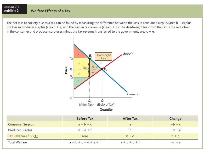
In Exhibit 2, we can now use consumer and producer surpluses to measure the amount of welfare loss associated with a tax. First, consider the amounts of consumer and producer surplus before the tax. Before the tax is imposed, the price is $P_1$ and the quantity is $Q_1$; at that price and output, the amount of consumer surplus is area $a+b+c$, and the amount of producer surplus is area $d+e+f$. To get the total surplus, or total welfare, we add consumer and producer surpluses, area $a+b+c+d+e+f$. Without $a$ tax, tax revenues are zero.

After the tax, the price the buyer pays is $P_B$, the price the seller receives is $P_s$, and the output falls to $Q_2$. As a result of the higher price and lower output from the tax, consumer surplus is smaller-area a. After the tax, sellers receive a lower price, so producer surplus is smaller-area f. However, some of the loss in consumer and producer surpluses is transferred in the form of tax revenues to the government, which can be used to reduce other taxes, fund public projects, or be redistributed to others in society. This transfer of society’s resources is not a loss from society’s perspective. The net loss to society can be found by measuring the difference between the loss in consumer surplus ( $a r e a b+c$ ) plus the loss in producer surplus (area $d+e$ ) and the gain in tax revenue $($ area $b+d)$. The reduction in total surplus is area $\mathrm{c}+\mathrm{e}$, or the shaded area in Exhibit 2. This deadweight loss from the tax is the reduction in producer and consumer surpluses minus the tax revenue transferred to the government.

经济代写|宏观经济学代考Macroeconomics代写|Elasticity and the Size of the Deadweight Loss

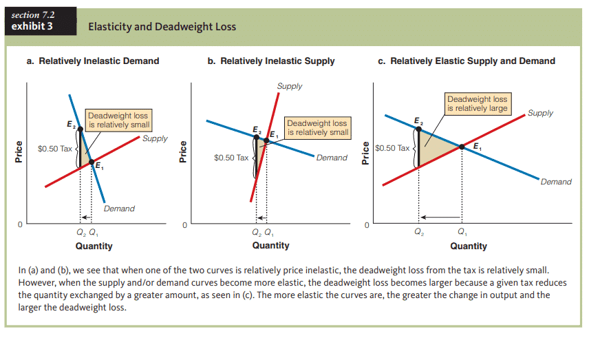
The size of the deadweight loss from a tax, as well as how the burdens are shared between buyers and sellers, depends on the price elasticities of supply and demand. In Exhibit 3(a) we can see that, other things being equal, the less elastic the demand curve, the smaller the deadweight loss. Similarly, the less elastic the supply curve, other things being equal, the smaller the deadweight loss, as shown in Exhibit 3(b). However, when the supply and/or demand curves become more elastic, the deadweight loss becomes larger because a given tax reduces the quantity exchanged by a greater amount, as seen in Exhibit 3(c). Recall that elasticities measure how responsive buyers and sellers are to price changes. That is, the more elastic the curves are, the greater the change in output and the larger the deadweight loss.

Elasticity differences can help us understand tax policy. Goods that are heavily taxed, such as alcohol, cigarettes, and gasoline, often have a relatively inelastic demand curve in the short run, so the tax burden falls primarily on the buyer. It also means that the deadweight loss to society is smaller for the tax revenue raised than if the demand curve were more elastic. In other words, because consumers cannot find many close substitutes in the short run, they reduce their consumption only slightly at the higher after-tax price. Even though the deadweight loss is smaller, it is still positive because the reduced after-tax price received by sellers and the increased after-tax price paid by buyers reduces the quantity exchanged below the previous market equilibrium level.

宏观经济学代写

经济代写|宏观经济学代考Macroeconomics代写|Using Consumer and Producer Surplus to Find the Welfare Effects of a Tax

为了简化对弹性和税收发生率的解释，我们不会像在第6.4节中那样移动供给曲线(向卖方征税)或需求曲线(向买方征税)，从而使说明复杂化。我们将简单地展示税收必然导致的结果。在新的税后产出下，供给曲线和需求曲线之间的垂直距离表示了税收，如图1中的粗体垂直线所示。税后，买方支付较高的价格$P_B$，卖方获得较低的价格$P_S$;商品的均衡量(包括买卖)从$Q_1$下降到$Q_2$。所征收的税收是通过将税额乘以征税后销售的货物数量来衡量的$\左(T \乘以Q_2\右)$。

在表2中，我们现在可以使用消费者和生产者剩余来衡量与税收相关的福利损失的数量。首先，考虑税前消费者和生产者剩余的数量。征税前，价格为$P_1$，数量为$Q_1$;在这个价格和产量下，消费者剩余的面积为a+b+c，生产者剩余的面积为d+e+f。为了得到总剩余或总福利，我们把消费者和生产者剩余加起来，面积a+b+c+d+e+f。没有$a$税，税收收入为零。

税后，买方支付的价格是$P_B$，卖方得到的价格是$P_s$，产量下降到$Q_2$。由于价格的提高和税收产出的减少，消费者剩余面积较小，面积为a。征税后，销售者得到的价格较低，因此生产者剩余面积较小。然而，消费者和生产者剩余的部分损失以税收的形式转移给政府，这些税收可以用来减少其他税收，资助公共项目，或者再分配给社会上的其他人。从社会的角度来看，这种社会资源的转移并不是一种损失。社会的净损失可以通过测量消费者剩余损失($ area b+c$)加上生产者剩余损失($ d+e$)和税收收入增加$($ area $b+d)$之间的差额来计算。总盈余的减少是面积$\ mathm {c}+\ mathm {e}$，或表2中的阴影区域。这种税收带来的无谓损失是生产者和消费者盈余的减少减去转移给政府的税收收入。

经济代写|宏观经济学代考Macroeconomics代写|Elasticity and the Size of the Deadweight Loss

税收带来的无谓损失的大小，以及买方和卖方如何分担负担，取决于供求的价格弹性。在图3(a)中我们可以看到，在其他条件相同的情况下，需求曲线的弹性越小，无谓损失越小。同样，在其他条件相同的情况下，供给曲线弹性越小，无谓损失越小，如图3(b)所示。然而，当供给和/或需求曲线变得更有弹性时，无谓损失变得更大，因为给定的税收减少了更大数量的交换量，如表3(c)所示。回想一下，弹性衡量的是买家和卖家对价格变化的反应程度。也就是说，曲线越有弹性，输出变化越大，自重损失越大。

弹性差异可以帮助我们理解税收政策。重税商品，如酒精、香烟和汽油，在短期内往往具有相对无弹性的需求曲线，因此税收负担主要落在买方身上。这也意味着，与需求曲线更具弹性的情况相比，增加税收对社会造成的无谓损失更小。换句话说，由于消费者在短期内找不到许多相近的替代品，他们只会以较高的税后价格略微减少消费。尽管无谓损失较小，但它仍然是正的，因为卖方获得的税后价格的减少和买方支付的税后价格的增加使交换量低于先前的市场均衡水平。

经济代写|宏观经济学代考Macroeconomics代写 请认准exambang™. exambang™为您的留学生涯保驾护航。

微观经济学代写

微观经济学是主流经济学的一个分支，研究个人和企业在做出有关稀缺资源分配的决策时的行为以及这些个人和企业之间的相互作用。my-assignmentexpert™ 为您的留学生涯保驾护航 在数学Mathematics作业代写方面已经树立了自己的口碑, 保证靠谱, 高质且原创的数学Mathematics代写服务。我们的专家在图论代写Graph Theory代写方面经验极为丰富，各种图论代写Graph Theory相关的作业也就用不着 说。

线性代数代写

线性代数是数学的一个分支，涉及线性方程，如：线性图，如：以及它们在向量空间和通过矩阵的表示。线性代数是几乎所有数学领域的核心。

博弈论代写

现代博弈论始于约翰-冯-诺伊曼（John von Neumann）提出的两人零和博弈中的混合策略均衡的观点及其证明。冯-诺依曼的原始证明使用了关于连续映射到紧凑凸集的布劳威尔定点定理，这成为博弈论和数学经济学的标准方法。在他的论文之后，1944年，他与奥斯卡-莫根斯特恩（Oskar Morgenstern）共同撰写了《游戏和经济行为理论》一书，该书考虑了几个参与者的合作游戏。这本书的第二版提供了预期效用的公理理论，使数理统计学家和经济学家能够处理不确定性下的决策。

微积分代写

微积分，最初被称为无穷小微积分或 “无穷小的微积分”，是对连续变化的数学研究，就像几何学是对形状的研究，而代数是对算术运算的概括研究一样。

它有两个主要分支，微分和积分；微分涉及瞬时变化率和曲线的斜率，而积分涉及数量的累积，以及曲线下或曲线之间的面积。这两个分支通过微积分的基本定理相互联系，它们利用了无限序列和无限级数收敛到一个明确定义的极限的基本概念 。

计量经济学代写

什么是计量经济学？
计量经济学是统计学和数学模型的定量应用，使用数据来发展理论或测试经济学中的现有假设，并根据历史数据预测未来趋势。它对现实世界的数据进行统计试验，然后将结果与被测试的理论进行比较和对比。

根据你是对测试现有理论感兴趣，还是对利用现有数据在这些观察的基础上提出新的假设感兴趣，计量经济学可以细分为两大类：理论和应用。那些经常从事这种实践的人通常被称为计量经济学家。

Matlab代写

MATLAB 是一种用于技术计算的高性能语言。它将计算、可视化和编程集成在一个易于使用的环境中，其中问题和解决方案以熟悉的数学符号表示。典型用途包括：数学和计算算法开发建模、仿真和原型制作数据分析、探索和可视化科学和工程图形应用程序开发，包括图形用户界面构建MATLAB 是一个交互式系统，其基本数据元素是一个不需要维度的数组。这使您可以解决许多技术计算问题，尤其是那些具有矩阵和向量公式的问题，而只需用 C 或 Fortran 等标量非交互式语言编写程序所需的时间的一小部分。MATLAB 名称代表矩阵实验室。MATLAB 最初的编写目的是提供对由 LINPACK 和 EISPACK 项目开发的矩阵软件的轻松访问，这两个项目共同代表了矩阵计算软件的最新技术。MATLAB 经过多年的发展，得到了许多用户的投入。在大学环境中，它是数学、工程和科学入门和高级课程的标准教学工具。在工业领域，MATLAB 是高效研究、开发和分析的首选工具。MATLAB 具有一系列称为工具箱的特定于应用程序的解决方案。对于大多数 MATLAB 用户来说非常重要，工具箱允许您学习和应用专业技术。工具箱是 MATLAB 函数（M 文件）的综合集合，可扩展 MATLAB 环境以解决特定类别的问题。可用工具箱的领域包括信号处理、控制系统、神经网络、模糊逻辑、小波、仿真等。