如果你也在 怎样代写神经网络Neural Networks AIML425这个学科遇到相关的难题,请随时右上角联系我们的24/7代写客服。神经网络Neural Networks理论既有助于更好地确定大脑中的神经元如何运作,也为创造人工智能的努力提供了基础。反映了人脑的行为,使计算机程序能够识别模式并解决人工智能、机器学习和深度学习领域的常见问题。
神经网络Neural Networks也被称为人工神经网络(ANN)或模拟神经网络(SNN),是机器学习的一个子集,是深度学习算法的核心。它们的名称和结构受到人脑的启发,模仿了生物神经元相互之间的信号方式。
my-assignmentexpert™ 神经网络Neural Networks作业代写,免费提交作业要求, 满意后付款,成绩80\%以下全额退款,安全省心无顾虑。专业硕 博写手团队,所有订单可靠准时,保证 100% 原创。my-assignmentexpert™, 最高质量的神经网络Neural Networks作业代写,服务覆盖北美、欧洲、澳洲等 国家。 在代写价格方面,考虑到同学们的经济条件,在保障代写质量的前提下,我们为客户提供最合理的价格。 由于统计Statistics作业种类很多,同时其中的大部分作业在字数上都没有具体要求,因此神经网络Neural Networks作业代写的价格不固定。通常在经济学专家查看完作业要求之后会给出报价。作业难度和截止日期对价格也有很大的影响。
想知道您作业确定的价格吗? 免费下单以相关学科的专家能了解具体的要求之后在1-3个小时就提出价格。专家的 报价比上列的价格能便宜好几倍。
my-assignmentexpert™ 为您的留学生涯保驾护航 在机器学习Machine Learning作业代写方面已经树立了自己的口碑, 保证靠谱, 高质且原创的机器学习Machine Learning代写服务。我们的专家在神经网络Neural Networks代写方面经验极为丰富,各种神经网络Neural Networks相关的作业也就用不着 说。
机器学习代写|神经网络代写Neural Networks代考|Best Matching Unit
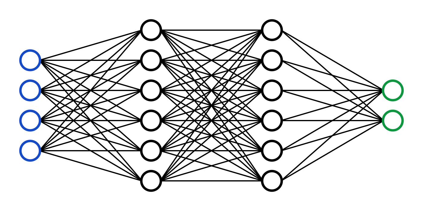
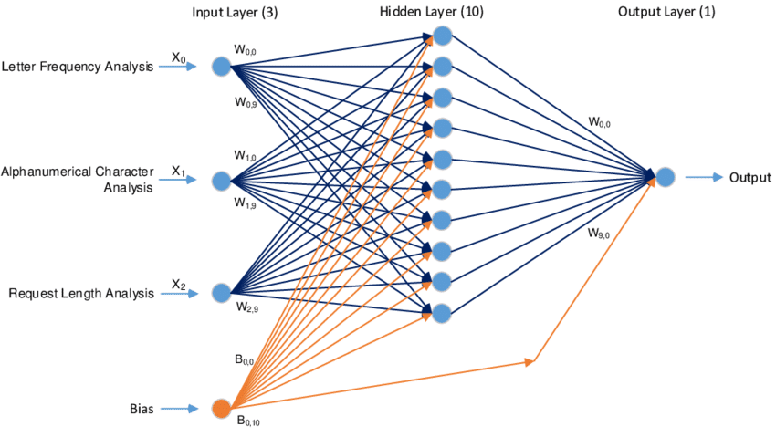
The Best Matehing Unit is the output neuron whose weights most closely match the input being provided to the neural network. Consider the SOM shown in Figure 8.1. There are 16 output neurons and 3 input neurons. This means that each of the 16 output neurons has 3 weights, one from each of the input neurons. The input to the SOM would also be three numbers, as there are three input neurons. To determine the BMU, we find the output neuron whose three weights most closely match the three input values fed into the SOM.
It is easy enough to calculate the BMU. To do this, we loop over every output neuron and calculate the Euclidean distance between the output neuron’s weights and the input values. The output neuron that has the lowest Euclidean distance is the BMU. The Euclidean distance is simply the distance between two multi-dimensional points. If you are dealing with two dimensions, the Euclidean distance is simply the length of a line drawn between the two points.
The Euclidean distance is used often in Machine Learning. It is a quick way to compare two arrays of numbers that have the same number of elements. Consider three arrays, named array $\mathbf{a}, \operatorname{array} \mathbf{b}$ and array $\mathbf{c}$. The Euclidean distance between array $\mathbf{a}$ and array $\mathbf{b}$ is 10 . The Euclidean distance between array a and array $\mathbf{c}$ is 20 . In this case, the contents of array a more closely match array $\mathbf{b}$ than they do array $\mathbf{c}$.
Equation 8.1 shows the formula for calculating the Euclidean distance.
Equation 8.1: The Euclidean Distance
$$
\mathrm{d}(\mathbf{p}, \mathbf{q})=\mathrm{d}(\mathbf{q}, \mathbf{p})=\sqrt{\left(q_1-p_1\right)^2+\left(q_2-p_2\right)^2+\cdots+\left(q_n-p_n\right)^2}=\sqrt{\sum_{i=1}^n\left(q_i-p_i\right)^2}
$$
The above equation shows us the Euclidean distance $\mathbf{d}$ between two arrays $\mathbf{p}$ and $\mathbf{q}$. The above equation also states that $\mathbf{d}(\mathbf{p}, \mathbf{q})$ is the same as $\mathbf{d}(\mathbf{q}, \mathbf{p})$. This simply means that the distance is the same no matter which end you start at. Calculation of the Euclidean distance is no more than summing the squares of the difference of each array element. Finally, the square root of this sum is taken. This square root is the Euclidean distance. The output neuron with the lowest Euclidean distance is the BMU.
机器学习代写|神经网络代写Neural Networks代考|Training a SOM
In the previous chapters, we learned several methods for training a feedforward neural network. We learned about such techniques as backpropagation, RPROP and LMA. These are all supervised training methods. Supervised training methods work by adjusting the weights of a neural network to produce the correct output for a given input.
A supervised training method will not work for a SOM. SOM networks require unsupervised training. In this section, we will learn to train a SOM with an unsupervised method. The training technique generally used for SOM networks is shown in Equation 8.2.
Equation 8.2: Training a SOM
$$
W_e(t+1)=W_v(t)+\theta(v, t) a(t)\left(D(t)-W_e(t)\right)
$$
The above equation shows how the weights of a SOM neural network are updated as training progresses. The current training iteration is noted by the letter $\mathbf{t}$, and the next training iteration is noted by $\mathbf{t}+\mathbf{1}$. Equation 8.2 allows us to see how weight $\mathbf{v}$ is adjusted for the next training iteration.
The variable $\mathbf{v}$ denotes that we are performing the same operation on every weight. The variable $\mathbf{W}$ represents the weights. The symbol theta is a special function, called a neighborhood function. The variable $\mathbf{D}$ represents the current training input to the SOM.
The symbol alpha denotes a learning rate. The learning rate changes for each iteration. This is why Equation 8.2 shows the learning rate with the symbol $\mathbf{t}$, as the learning rate is attached to the iteration. The learning rate for a SOM is said to be monotonically decreasing. Monotonically decreasing means that the learning rate only falls, and never increases.
神经网络代写
机器学习代写|神经网络代写Neural Networks代考|Best Matching Unit
最佳匹配单元是输出神经元,其权重与提供给神经网络的输入最接近。考虑图8.1所示的SOM。有16个输出神经元和3个输入神经元。这意味着16个输出神经元中的每一个都有3个权重,每个权重来自输入神经元。SOM的输入也是三个数字,因为有三个输入神经元。为了确定BMU,我们找到三个权重最接近于输入到SOM的三个输入值的输出神经元。
计算BMU很简单。为了做到这一点,我们循环遍历每个输出神经元,并计算输出神经元的权重和输入值之间的欧几里德距离。欧几里得距离最小的输出神经元是BMU。欧几里得距离就是两个多维点之间的距离。如果是在二维空间中,欧几里得距离就是两点之间的直线长度。
欧几里得距离在机器学习中经常使用。这是比较两个具有相同元素数量的数字数组的一种快速方法。考虑三个数组,分别名为array $\mathbf{a}, \operatorname{array} \mathbf{b}$和array $\mathbf{c}$。阵列$\mathbf{a}$与阵列$\mathbf{b}$之间的欧氏距离为10。数组a和数组$\mathbf{c}$之间的欧氏距离为20。在这种情况下,数组a的内容更接近于匹配数组$\mathbf{b}$而不是数组$\mathbf{c}$。
欧几里得距离的计算公式如式8.1所示。
式8.1:欧几里得距离
$$
\mathrm{d}(\mathbf{p}, \mathbf{q})=\mathrm{d}(\mathbf{q}, \mathbf{p})=\sqrt{\left(q_1-p_1\right)^2+\left(q_2-p_2\right)^2+\cdots+\left(q_n-p_n\right)^2}=\sqrt{\sum_{i=1}^n\left(q_i-p_i\right)^2}
$$
上面的等式显示了两个数组$\mathbf{p}$和$\mathbf{q}$之间的欧几里得距离$\mathbf{d}$。上面的等式还表明$\mathbf{d}(\mathbf{p}, \mathbf{q})$等于$\mathbf{d}(\mathbf{q}, \mathbf{p})$。这仅仅意味着无论你从哪一端出发,距离都是一样的。欧几里得距离的计算只不过是对每个阵列元素的差的平方求和。最后,取这个和的平方根。这个平方根就是欧几里得距离。欧几里得距离最小的输出神经元是BMU。
机器学习代写|神经网络代写Neural Networks代考|Training a SOM
在前面的章节中,我们学习了训练前馈神经网络的几种方法。我们学习了反向传播、RPROP和LMA等技术。这些都是有监督的训练方法。监督训练方法通过调整神经网络的权重来产生给定输入的正确输出。
有监督的培训方法不适用于高级管理人员。SOM网络需要无监督的训练。在本节中,我们将学习用无监督的方法训练SOM。一般用于SOM网络的训练技术如式8.2所示。
方程8.2:训练SOM
$$
W_e(t+1)=W_v(t)+\theta(v, t) a(t)\left(D(t)-W_e(t)\right)
$$
上面的方程显示了SOM神经网络的权值是如何随着训练的进行而更新的。当前的训练迭代用字母$\mathbf{t}$表示,下一个训练迭代用字母$\mathbf{t}+\mathbf{1}$表示。公式8.2允许我们看到权重$\mathbf{v}$是如何为下一次训练迭代进行调整的。
变量$\mathbf{v}$表示我们对每个权重执行相同的操作。变量$\mathbf{W}$表示权重。符号是一个特殊的函数,叫做邻域函数。变量$\mathbf{D}$表示当前对SOM的训练输入。
符号alpha表示学习率。每次迭代的学习率都会发生变化。这就是为什么公式8.2用符号$\mathbf{t}$表示学习率,因为学习率是附加在迭代上的。SOM的学习率是单调递减的。单调递减意味着学习率只会下降,不会增加。

机器学习代写|神经网络代写Neural Networks代考 请认准UprivateTA™. UprivateTA™为您的留学生涯保驾护航。
微观经济学代写
微观经济学是主流经济学的一个分支,研究个人和企业在做出有关稀缺资源分配的决策时的行为以及这些个人和企业之间的相互作用。my-assignmentexpert™ 为您的留学生涯保驾护航 在数学Mathematics作业代写方面已经树立了自己的口碑, 保证靠谱, 高质且原创的数学Mathematics代写服务。我们的专家在图论代写Graph Theory代写方面经验极为丰富,各种图论代写Graph Theory相关的作业也就用不着 说。
线性代数代写
线性代数是数学的一个分支,涉及线性方程,如:线性图,如:以及它们在向量空间和通过矩阵的表示。线性代数是几乎所有数学领域的核心。
博弈论代写
现代博弈论始于约翰-冯-诺伊曼(John von Neumann)提出的两人零和博弈中的混合策略均衡的观点及其证明。冯-诺依曼的原始证明使用了关于连续映射到紧凑凸集的布劳威尔定点定理,这成为博弈论和数学经济学的标准方法。在他的论文之后,1944年,他与奥斯卡-莫根斯特恩(Oskar Morgenstern)共同撰写了《游戏和经济行为理论》一书,该书考虑了几个参与者的合作游戏。这本书的第二版提供了预期效用的公理理论,使数理统计学家和经济学家能够处理不确定性下的决策。
微积分代写
微积分,最初被称为无穷小微积分或 “无穷小的微积分”,是对连续变化的数学研究,就像几何学是对形状的研究,而代数是对算术运算的概括研究一样。
它有两个主要分支,微分和积分;微分涉及瞬时变化率和曲线的斜率,而积分涉及数量的累积,以及曲线下或曲线之间的面积。这两个分支通过微积分的基本定理相互联系,它们利用了无限序列和无限级数收敛到一个明确定义的极限的基本概念 。
计量经济学代写
什么是计量经济学?
计量经济学是统计学和数学模型的定量应用,使用数据来发展理论或测试经济学中的现有假设,并根据历史数据预测未来趋势。它对现实世界的数据进行统计试验,然后将结果与被测试的理论进行比较和对比。
根据你是对测试现有理论感兴趣,还是对利用现有数据在这些观察的基础上提出新的假设感兴趣,计量经济学可以细分为两大类:理论和应用。那些经常从事这种实践的人通常被称为计量经济学家。
MATLAB代写
MATLAB 是一种用于技术计算的高性能语言。它将计算、可视化和编程集成在一个易于使用的环境中,其中问题和解决方案以熟悉的数学符号表示。典型用途包括:数学和计算算法开发建模、仿真和原型制作数据分析、探索和可视化科学和工程图形应用程序开发,包括图形用户界面构建MATLAB 是一个交互式系统,其基本数据元素是一个不需要维度的数组。这使您可以解决许多技术计算问题,尤其是那些具有矩阵和向量公式的问题,而只需用 C 或 Fortran 等标量非交互式语言编写程序所需的时间的一小部分。MATLAB 名称代表矩阵实验室。MATLAB 最初的编写目的是提供对由 LINPACK 和 EISPACK 项目开发的矩阵软件的轻松访问,这两个项目共同代表了矩阵计算软件的最新技术。MATLAB 经过多年的发展,得到了许多用户的投入。在大学环境中,它是数学、工程和科学入门和高级课程的标准教学工具。在工业领域,MATLAB 是高效研究、开发和分析的首选工具。MATLAB 具有一系列称为工具箱的特定于应用程序的解决方案。对于大多数 MATLAB 用户来说非常重要,工具箱允许您学习和应用专业技术。工具箱是 MATLAB 函数(M 文件)的综合集合,可扩展 MATLAB 环境以解决特定类别的问题。可用工具箱的领域包括信号处理、控制系统、神经网络、模糊逻辑、小波、仿真等。