0 0

By admin Statistical inference 统计统计代写统计推断 2023年8月28日

代写隐藏

1 统计代写|统计推断代考Statistical Inference代写|Definition of Probability and Some Basic Results

2 统计代写|统计推断代考Statistical Inference代写|RELATIVE FREQUENCY DEFINITION OF PROBABILITY

3 统计推断代写

3.1 统计代写|统计推断代考Statistical Inference代写|Definition of Probability and Some Basic Results

3.2 统计代写|统计推断代考Statistical Inference代写|RELATIVE FREQUENCY DEFINITION OF PROBABILITY

如果你也在怎样代写统计推断Statistical Inference 这个学科遇到相关的难题，请随时右上角联系我们的24/7代写客服。统计推断Statistical Inference领域，有两种主要的思想流派。每一种方法都有其支持者，但人们普遍认为，在入门课程中涵盖的所有问题上，这两种方法都是有效的，并且在应用于实际问题时得到相同的数值。传统课程只涉及其中一种方法，这使得学生无法接触到统计推断的整个领域。传统的方法，也被称为频率论或正统观点，几乎直接导致了上面的问题。另一种方法，也称为概率论作为逻辑${}^1$，直接从概率论导出所有统计推断。

统计推断Statistical Inference指的是一个研究领域，我们在面对不确定性的情况下，根据我们观察到的数据，试图推断世界的未知特性。它是一个数学框架，在许多情况下量化我们的常识所说的话，但在常识不够的情况下，它允许我们超越常识。对正确的统计推断的无知会导致错误的决策和浪费金钱。就像对其他领域的无知一样，对统计推断的无知也会让别人操纵你，让你相信一些错误的事情是正确的。

统计推断Statistical Inference代写，免费提交作业要求，满意后付款，成绩80\%以下全额退款，安全省心无顾虑。专业硕博写手团队，所有订单可靠准时，保证 100% 原创。最高质量的统计推断Statistical Inference作业代写，服务覆盖北美、欧洲、澳洲等国家。在代写价格方面，考虑到同学们的经济条件，在保障代写质量的前提下，我们为客户提供最合理的价格。由于作业种类很多，同时其中的大部分作业在字数上都没有具体要求，因此统计推断Statistical Inference作业代写的价格不固定。通常在专家查看完作业要求之后会给出报价。作业难度和截止日期对价格也有很大的影响。

同学们在留学期间，都对各式各样的作业考试很是头疼，如果你无从下手，不如考虑my-assignmentexpert™！

my-assignmentexpert™提供最专业的一站式服务：Essay代写，Dissertation代写，Assignment代写，Paper代写，Proposal代写，Proposal代写，Literature Review代写，Online Course，Exam代考等等。my-assignmentexpert™专注为留学生提供Essay代写服务，拥有各个专业的博硕教师团队帮您代写，免费修改及辅导，保证成果完成的效率和质量。同时有多家检测平台帐号，包括Turnitin高级账户，检测论文不会留痕，写好后检测修改，放心可靠，经得起任何考验！

统计代写|统计推断代考Statistical Inference代写|STAT4027

统计代写|统计推断代考Statistical Inference代写|Definition of Probability and Some Basic Results

When a random experiment is entertained, one of the first questions which arise is, what is the probability that a certain event occurs? For instance, in reference to Example 26 in Chapter 1, one may ask: What is the probability that exactly one head occurs; in other words, what is the probability of the event $B={H T T, T H T, T T H}$ ? The answer to this question is almost automatic and is $3 / 8$. The relevant reasoning goes like this: Assuming that the three coins are balanced, the probability of each one of the 8 outcomes, considered as simple events, must be $1 / 8$. Since the event $B$ consists of 3 sample points, it can occur in 3 different ways, and hence its probability must be $3 / 8$.

This is exactly the intuitive reasoning employed in defining the concept of probability when two requirements are met: First, the sample space $\mathcal{S}$ has finitely many outcomes, $\mathcal{S}=\left{s_1, \ldots, s_n\right}$, say, and second, each one of these outcomes is “equally likely” to occur, has the same chance of appearing, whenever the relevant random experiment is carried out. This reasoning is based on the underlying symmetry. Thus, one is led to stipulating that each one of the (simple) events $\left{s_i\right}, i=1, \ldots, n$ has probability $1 / n$. Then the next step, that of defining the probability of a composite event $A$, is simple; if $A$ consists of $m$ sample points, $A=\left{s_{i_1}, \ldots, s_{i_m}\right}$, say $(1 \leq m \leq n)$ (or none at all, in which case $m=0$ ), then the probability of $A$ must be $m / n$. The notation used is: $P\left(\left{s_1\right}\right)=\cdots=P\left(\left{s_n\right}\right)=\frac{1}{n}$ and $P(A)=\frac{m}{n}$. Actually, this is the so-called classical definition of probability. That is,

CLASSICAL DEFINITION OF PROBABILITY Let $\mathcal{S}$ be a sample space, associated with a certain random experiment and consisting of finitely many sample points $n$, say, each of which is equally likely to occur whenever the random experiment is carried out. Then the probability of any event $A$, consisting of $m$ sample points $(0 \leq m \leq n)$, is given by $P(A)=\frac{m}{n}$.

In reference to Example 26 in Chapter $1, P(A)=\frac{4}{8}=\frac{1}{2}=0.5$. In Example 27 (when the two dice are unbiased), $P(X=7)=\frac{6}{36}=\frac{1}{6} \simeq 0.167$, where the r.v. $X$ and the event $(X=7)$ are defined in Section 1.3. In Example 29, when the balls in the urn are thoroughly mixed, we may assume that all of the $(m+n)(m+n-1)$ pairs are equally likely to be selected. Then, since the event $A$ occurs in 20 different ways, $P(A)=\frac{20}{(m+n)(m+n-1)}$. For $m=3$ and $n=5$, this probability is $P(A)=\frac{20}{56}=\frac{5}{14} \simeq 0.357$.

From the preceding (classical) definition of probability, the following simple properties are immediate: For any event $A, P(A) \geq 0 ; P(\mathcal{S})=1$; if two events $A_1$ and $A_2$ are disjoint $\left(A_1 \cap A_2=\varnothing\right)$, then $P\left(A_1 \cup A_2\right)=P\left(A_1\right)+P\left(A_2\right)$. This is so because, if $A_1=\left{s_{i_1}, \ldots, s_{i_k}\right}, A_2=\left{s_{j_1}, \ldots, s_{j_{\ell}}\right}$, where all $s_{i_1}, \ldots, s_{i_k}$ are distinct from all $s_{j_1}, \ldots, s_{j_{\ell}}$, then $A_1 \cup A_2=\left{s_{i_1}, \ldots, s_{i_k} s_{j_1}, \ldots, s_{j_{\ell}}\right}$ and $P\left(A_1 \cup A_2\right)=\frac{k+\ell}{n}=\frac{k}{n}+\frac{\ell}{n}=P\left(A_1\right)+P\left(A_2\right)$.

统计代写|统计推断代考Statistical Inference代写|RELATIVE FREQUENCY DEFINITION OF PROBABILITY

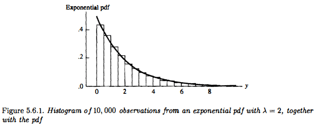
Let $N(A)$ be the number of times an event $A$ occurs in $N$ repetitions of a random experiment, and assume that the relative frequency of $A, \frac{N(A)}{N}$, converges to a limit as $N \rightarrow \infty$. This limit is denoted by $P(A)$ and is called the probability of $A$.

At this point, it is to be observed that empirical data show that the relative frequency definition of probability and the classical definition of probability agree in the framework in which the classical definition applies.

From the relative frequency definition of probability and the usual properties of limits, it is immediate that: $P(A) \geq 0$ for every event $A ; P(S)=1$; and for $A_1, A_2$ with $A_1 \cap A_2=\varnothing$,
$$
\begin{aligned}
P\left(A_1 \cup A_2\right) & =\lim {N \rightarrow \infty} \frac{N\left(A_1 \cup A_2\right)}{N}=\lim {N \rightarrow \infty}\left(\frac{N\left(A_1\right)}{N}+\frac{N\left(A_2\right)}{N}\right) \
& =\lim {N \rightarrow \infty} \frac{N\left(A_1\right)}{N}+\lim {N \rightarrow \infty} \frac{N\left(A_2\right)}{N}=P\left(A_1\right)+P\left(A_2\right) ;
\end{aligned}
$$
that is, $P\left(A_1 \cup A_2\right)=P\left(A_1\right)+P\left(A_2\right)$, provided $A_1 \cap A_2=\varnothing$. These three properties were also seen to be true in the classical definition of probability. Furthermore, it is immediate that under either definition of probability, $P\left(A_1 \cup \ldots \cup A_k\right)=P\left(A_1\right)+\cdots+P\left(A_k\right)$, provided the events are pairwise disjoint; $A_i \cap A_j=\varnothing, i \neq j$.

The above two definitions of probability certainly give substance to the concept of probability in a way consonant with our intuition about what probability should be. However, for the purpose of cultivating the concept and deriving deep probabilistic results, one must define the concept of probability in terms of some basic properties, which would not contradict what we have seen so far. This line of thought leads to the so-called axiomatic definition of probability due to Kolmogorov.

统计推断代写

统计代写|统计推断代考Statistical Inference代写|Definition of Probability and Some Basic Results

当进行随机实验时，首先出现的问题之一是，某一事件发生的概率是多少?例如，参考第一章例26，人们可能会问:恰好出现一个正面的概率是多少?换句话说，事件$B={H T T, T H T, T T H}$的概率是多少?这个问题的答案几乎是自动的，是$3 / 8$。相关的推理是这样的:假设三个硬币是平衡的，那么作为简单事件的8种结果中的每一种的概率必须是$1 / 8$。由于事件$B$由3个样本点组成，它可以以3种不同的方式发生，因此它的概率必须为$3 / 8$。

这正是在满足两个要求时定义概率概念时所采用的直观推理:首先，样本空间$\mathcal{S}$具有有限多个结果，例如$\mathcal{S}=\left{s_1, \ldots, s_n\right}$;其次，无论何时进行相关的随机实验，这些结果中的每一个都“等可能”发生，出现的机会相同。这种推理是基于潜在的对称性。这样，人们就会规定每个(简单)事件$\left{s_i\right}, i=1, \ldots, n$都有概率$1 / n$。那么下一步，即定义复合事件$A$的概率，就很简单了;如果$A$包含$m$个样本点，$A=\left{s_{i_1}, \ldots, s_{i_m}\right}$，比如$(1 \leq m \leq n)$(或者根本没有，在这种情况下$m=0$)，那么$A$的概率一定是$m / n$。使用的符号是:$P\left(\left{s_1\right}\right)=\cdots=P\left(\left{s_n\right}\right)=\frac{1}{n}$和$P(A)=\frac{m}{n}$。实际上，这就是所谓的概率的经典定义。也就是说，

设$\mathcal{S}$是一个样本空间，它与某个随机实验相关联，由有限个样本点组成$n$，例如，在进行随机实验时，每个样本点出现的可能性都是相等的。由$m$个样本点$(0 \leq m \leq n)$组成的任意事件$A$的概率由$P(A)=\frac{m}{n}$给出。

参考$1, P(A)=\frac{4}{8}=\frac{1}{2}=0.5$章例26。在例27中(当两个骰子是无偏的)，$P(X=7)=\frac{6}{36}=\frac{1}{6} \simeq 0.167$，其中rv $X$和事件$(X=7)$在第1.3节中定义。在例29中，当瓮中的球完全混合时，我们可以假设所有$(m+n)(m+n-1)$对被选中的可能性相等。然后，由于事件$A$以20种不同的方式发生，$P(A)=\frac{20}{(m+n)(m+n-1)}$。对于$m=3$和$n=5$，这个概率是$P(A)=\frac{20}{56}=\frac{5}{14} \simeq 0.357$。

从前面的(经典的)概率定义，下列简单的性质是直接的:对于任何事件$A, P(A) \geq 0 ; P(\mathcal{S})=1$;如果两个事件$A_1$和$A_2$不相交$\left(A_1 \cap A_2=\varnothing\right)$，则$P\left(A_1 \cup A_2\right)=P\left(A_1\right)+P\left(A_2\right)$。这是因为，如果$A_1=\left{s_{i_1}, \ldots, s_{i_k}\right}, A_2=\left{s_{j_1}, \ldots, s_{j_{\ell}}\right}$，其中所有的$s_{i_1}, \ldots, s_{i_k}$都不同于所有的$s_{j_1}, \ldots, s_{j_{\ell}}$，那么$A_1 \cup A_2=\left{s_{i_1}, \ldots, s_{i_k} s_{j_1}, \ldots, s_{j_{\ell}}\right}$和$P\left(A_1 \cup A_2\right)=\frac{k+\ell}{n}=\frac{k}{n}+\frac{\ell}{n}=P\left(A_1\right)+P\left(A_2\right)$。

统计代写|统计推断代考Statistical Inference代写|RELATIVE FREQUENCY DEFINITION OF PROBABILITY

设$N(A)$为一个事件$A$在一个随机实验的$N$次重复中出现的次数，并假设$A, \frac{N(A)}{N}$的相对频率收敛到一个极限$N \rightarrow \infty$。这个极限用$P(A)$表示，称为$A$的概率。

在这一点上，值得注意的是，经验数据表明，概率的相对频率定义和概率的经典定义在经典定义适用的框架内是一致的。

从概率的相对频率定义和极限的通常性质来看，可以直接得到:$P(A) \geq 0$对于每一个事件$A ; P(S)=1$;对于$A_1, A_2$和$A_1 \cap A_2=\varnothing$，
$$
\begin{aligned}
P\left(A_1 \cup A_2\right) & =\lim {N \rightarrow \infty} \frac{N\left(A_1 \cup A_2\right)}{N}=\lim {N \rightarrow \infty}\left(\frac{N\left(A_1\right)}{N}+\frac{N\left(A_2\right)}{N}\right) \
& =\lim {N \rightarrow \infty} \frac{N\left(A_1\right)}{N}+\lim {N \rightarrow \infty} \frac{N\left(A_2\right)}{N}=P\left(A_1\right)+P\left(A_2\right) ;
\end{aligned}
$$
即$P\left(A_1 \cup A_2\right)=P\left(A_1\right)+P\left(A_2\right)$，提供$A_1 \cap A_2=\varnothing$。这三个性质在概率的经典定义中也被认为是正确的。此外，在任意一个概率定义$P\left(A_1 \cup \ldots \cup A_k\right)=P\left(A_1\right)+\cdots+P\left(A_k\right)$下，只要事件是两两不相交的;$A_i \cap A_j=\varnothing, i \neq j$。

概率的上述两种定义确实以一种与我们关于概率应该是什么的直觉一致的方式赋予了概率概念实质。然而，为了培养这个概念并得出深层次的概率结果，我们必须根据一些基本性质来定义概率的概念，这与我们目前所看到的并不矛盾。这种思路导致了Kolmogorov提出的所谓概率的公理化定义。

统计代写|统计推断代考Statistical Inference代写请认准exambang™. exambang™为您的留学生涯保驾护航。

微观经济学代写

微观经济学是主流经济学的一个分支，研究个人和企业在做出有关稀缺资源分配的决策时的行为以及这些个人和企业之间的相互作用。my-assignmentexpert™ 为您的留学生涯保驾护航在数学Mathematics作业代写方面已经树立了自己的口碑, 保证靠谱, 高质且原创的数学Mathematics代写服务。我们的专家在图论代写Graph Theory代写方面经验极为丰富，各种图论代写Graph Theory相关的作业也就用不着说。

线性代数代写

线性代数是数学的一个分支，涉及线性方程，如：线性图，如：以及它们在向量空间和通过矩阵的表示。线性代数是几乎所有数学领域的核心。

博弈论代写

现代博弈论始于约翰-冯-诺伊曼（John von Neumann）提出的两人零和博弈中的混合策略均衡的观点及其证明。冯-诺依曼的原始证明使用了关于连续映射到紧凑凸集的布劳威尔定点定理，这成为博弈论和数学经济学的标准方法。在他的论文之后，1944年，他与奥斯卡-莫根斯特恩（Oskar Morgenstern）共同撰写了《游戏和经济行为理论》一书，该书考虑了几个参与者的合作游戏。这本书的第二版提供了预期效用的公理理论，使数理统计学家和经济学家能够处理不确定性下的决策。

微积分代写

微积分，最初被称为无穷小微积分或 “无穷小的微积分”，是对连续变化的数学研究，就像几何学是对形状的研究，而代数是对算术运算的概括研究一样。

它有两个主要分支，微分和积分；微分涉及瞬时变化率和曲线的斜率，而积分涉及数量的累积，以及曲线下或曲线之间的面积。这两个分支通过微积分的基本定理相互联系，它们利用了无限序列和无限级数收敛到一个明确定义的极限的基本概念。

计量经济学代写

什么是计量经济学？
计量经济学是统计学和数学模型的定量应用，使用数据来发展理论或测试经济学中的现有假设，并根据历史数据预测未来趋势。它对现实世界的数据进行统计试验，然后将结果与被测试的理论进行比较和对比。

根据你是对测试现有理论感兴趣，还是对利用现有数据在这些观察的基础上提出新的假设感兴趣，计量经济学可以细分为两大类：理论和应用。那些经常从事这种实践的人通常被称为计量经济学家。

Matlab代写

MATLAB 是一种用于技术计算的高性能语言。它将计算、可视化和编程集成在一个易于使用的环境中，其中问题和解决方案以熟悉的数学符号表示。典型用途包括：数学和计算算法开发建模、仿真和原型制作数据分析、探索和可视化科学和工程图形应用程序开发，包括图形用户界面构建MATLAB 是一个交互式系统，其基本数据元素是一个不需要维度的数组。这使您可以解决许多技术计算问题，尤其是那些具有矩阵和向量公式的问题，而只需用 C 或 Fortran 等标量非交互式语言编写程序所需的时间的一小部分。MATLAB 名称代表矩阵实验室。MATLAB 最初的编写目的是提供对由 LINPACK 和 EISPACK 项目开发的矩阵软件的轻松访问，这两个项目共同代表了矩阵计算软件的最新技术。MATLAB 经过多年的发展，得到了许多用户的投入。在大学环境中，它是数学、工程和科学入门和高级课程的标准教学工具。在工业领域，MATLAB 是高效研究、开发和分析的首选工具。MATLAB 具有一系列称为工具箱的特定于应用程序的解决方案。对于大多数 MATLAB 用户来说非常重要，工具箱允许您学习和应用专业技术。工具箱是 MATLAB 函数（M 文件）的综合集合，可扩展 MATLAB 环境以解决特定类别的问题。可用工具箱的领域包括信号处理、控制系统、神经网络、模糊逻辑、小波、仿真等。