如果你也在 怎样代写统计推断Statistical Inference 这个学科遇到相关的难题，请随时右上角联系我们的24/7代写客服。统计推断Statistical Inference是利用数据分析来推断概率基础分布的属性的过程。推断性统计分析推断人口的属性，例如通过测试假设和得出估计值。假设观察到的数据集是从一个更大的群体中抽出的。

统计推断Statistical Inference（可以与描述性统计进行对比。描述性统计只关注观察到的数据的属性，它并不依赖于数据来自一个更大的群体的假设。在机器学习中，推理一词有时被用来代替 “通过评估一个已经训练好的模型来进行预测”；在这种情况下，推断模型的属性被称为训练或学习（而不是推理），而使用模型进行预测被称为推理（而不是预测）；另见预测推理。

统计推断Statistical Inference代写，免费提交作业要求， 满意后付款，成绩80\%以下全额退款，安全省心无顾虑。专业硕 博写手团队，所有订单可靠准时，保证 100% 原创。最高质量的统计推断Statistical Inference作业代写，服务覆盖北美、欧洲、澳洲等 国家。 在代写价格方面，考虑到同学们的经济条件，在保障代写质量的前提下，我们为客户提供最合理的价格。 由于作业种类很多，同时其中的大部分作业在字数上都没有具体要求，因此统计推断Statistical Inference作业代写的价格不固定。通常在专家查看完作业要求之后会给出报价。作业难度和截止日期对价格也有很大的影响。

同学们在留学期间，都对各式各样的作业考试很是头疼，如果你无从下手，不如考虑my-assignmentexpert™！

my-assignmentexpert™提供最专业的一站式服务：Essay代写，Dissertation代写，Assignment代写，Paper代写，Proposal代写，Proposal代写，Literature Review代写，Online Course，Exam代考等等。my-assignmentexpert™专注为留学生提供Essay代写服务，拥有各个专业的博硕教师团队帮您代写，免费修改及辅导，保证成果完成的效率和质量。同时有多家检测平台帐号，包括Turnitin高级账户，检测论文不会留痕，写好后检测修改，放心可靠，经得起任何考验！

统计代写|统计推断代考Statistical Inference代写|Basics of Probability Theory

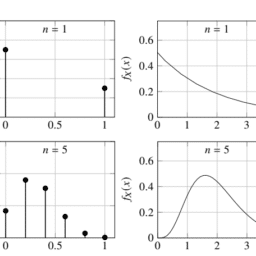
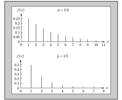
When an experiment is performed, the realization of the experiment is an outcome in the sample space. If the experiment is performed a number of times, different outcomes may occur each time or some outcomes may repeat. This “frequency of occurrence” of an outcome can be thought of as a probability. More probable outcomes occur more frequently. If the outcomes of an experiment can be described probabilistically, we are on our way to analyzing the experiment statistically.
In this section we describe some of the basics of probability theory. We do not define probabilities in terms of frequencies but instead take the mathematically simpler axiomatic approach. As will be seen, the axiomatic approach is not concerned with the interpretations of probabilities, but is concerned only that the probabilities are defined by a function satisfying the axioms. Interpretations of the probabilities are quite another matter. The “frequency of occurrence” of an event is one example of a particular interpretation of probability. Another possible interpretation is a subjective one, where rather than thinking of probability as frequency, we can think of it as a belief in the chance of an event occurring.
Axiomatic Foundations
For each event $A$ in the sample space $S$ we want to associate with $A$ a number between zero and one that will be called the probability of $A$, denoted by $P(A)$. It would seem natural to define the domain of $P$ (the set where the arguments of the function $P(\cdot)$ are defined) as all subsets of $S$; that is, for each $A \subset S$ we define $P(A)$ as the probability that $A$ occurs. Unfortunately, matters are not that simple. There are some technical difficulties to overcome. We will not dwell on these technicalities; although they are of importance, they are usually of more interest to probabilists than to statisticians. However, a firm understanding of statistics requires at least a passing familiarity with the following.
Definition 1.2.1 A collection of subsets of $S$ is called a sigma algebra (or Borel field), denoted by $\mathcal{B}$, if it satisfies the following three properties:
a. $\emptyset \in \mathcal{B}$ (the empty set is an element of $\mathcal{B}$ ).
b. If $A \in \mathcal{B}$, then $A^{\mathrm{c}} \in \mathcal{B}$ ( $\mathcal{B}$ is closed under complementation).
c. If $A_1, A_2, \ldots \in \mathcal{B}$, then $\cup_{i=1}^{\infty} A_i \in \mathcal{B}$ ( $\mathcal{B}$ is closed under countable unions).
The empty set $\emptyset$ is a subset of any set. Thus, $\emptyset \subset S$. Property (a) states that this subset is always in a sigma algebra. Since $S=\emptyset^c$, properties (a) and (b) imply that $S$ is always in $\mathcal{B}$ also. In addition, from DeMorgan’s Laws it follows that $\mathcal{B}$ is closed under countable intersections.’ If $A_1, A_2, \ldots \in \mathcal{B}$, then $A_1^c, A_2^c, \ldots \in \mathcal{B}$ by property (b), and therefore $\cup_{i=1}^{\infty} A_i^c \in \mathcal{B}$. However, using DeMorgan’s Law (as in Exercise 1.9), we have
$$
\left(\bigcup_{i=1}^{\infty} A_i^c\right)^{\mathrm{c}}=\bigcap_{i=1}^{\infty} A_i .
$$
Thus, again by property (b), $\cap_{i=1}^{\infty} A_i \in \mathcal{B}$.
Associated with sample space $S$ we can have many different sigma algebras. For example, the collection of the two sets ${\emptyset, S}$ is a sigma algebra, usually called the trivial sigma algebra. The only sigma algebra we will be concerned with is the smallest one that contains all of the open sets in a given sample space $S$.

统计代写|统计推断代考Statistical Inference代写|The Calculus of Probabilities

From the Axioms of Probability we can build up many properties of the probability – function, properties that are quite helpful in the calculation of more complicated probabilities. Some of these manipulations will be discussed in detail in this section; others will be left as exercises.
We start with some (fairly self-evident) properties of the probability function when applied to a single event.
Theorem 1.2.8 If $P$ is a probability function and $A$ is any set in $\mathcal{B}$, then
a. $P(\emptyset)=0$, where $\emptyset$ is the empty set;
b. $P(A) \leq 1$;
c. $P\left(A^{\mathrm{c}}\right)=1-P(A)$.
Proof: It is easiest to prove (c) first. The sets $A$ and $A^c$ form a partition of the sample space, that is, $S=A \cup A^c$. Therefore,
$$
P\left(A \cup A^c\right)=P(S)=1
$$
by the second axiom. Also, $A$ and $A^c$ are disjoint, so by the third axiom,
$$
P\left(A \cup A^c\right)=P(A)+P\left(A^c\right)
$$
Combining (1.2.4) and (1.2.5) gives (c).
Since $P\left(A^c\right) \geq 0$, (b) is immediately implied by (c). To prove (a), we use a similar argument on $S=S \cup \emptyset$. (Recall that both $S$ and $\emptyset$ are always in $\mathcal{B}$.) Since $S$ and $\emptyset$ are disjoint, we have
$$
1=P(S)=P(S \cup \emptyset)=P(S)+P(\emptyset)
$$
and thus $P(\theta)=0$
Theorem 1.2 .8 contains properties that are so basic that they also have the flavor of axioms, although we have formally proved them using only the original three Kolmogorov Axioms. The next theorem, which is similar in spirit to Theorem 1.2.8, contains statements that are not so self-evident.
Theorem 1.2.9 If $P$ is a probability function and $A$ and $B$ are any sets in $B$, then a. $P\left(B \cap A^c\right)=P(B)-P(A \cap B)$;
b. $P(A \cup B)=P(A)+P(B)-P(A \cap B)$;
c. If $A \subset B$, then $P(A) \leq P(B)$.
Proof: To establish (a) note that for any sets $A$ and $B$ we have
$$
B={B \cap A} \cup\left{B \cap A^c\right}
$$
and therefore
$$
P(B)=P\left({B \cap A} \cup\left{B \cap A^c\right}\right)=P(B \cap A)+P\left(B \cap A^{\mathrm{c}}\right)
$$
where the last equality in (1.2.6) follows from the fact that $B \cap A$ and $B \cap A^c$ are disjoint. Rearranging (1.2.6) gives (a).
To establish (b), we use the identity
$$
A \cup B=A \cup\left{B \cap A^{\mathrm{c}}\right}
$$

统计推断代写

统计代写|统计推断代考Statistical Inference代写|Basics of Probability Theory

当进行实验时，实验的实现是样本空间中的结果。如果实验进行多次，每次可能出现不同的结果，或者有些结果可能重复。一个结果的“出现频率”可以被认为是概率。更可能的结果更频繁地出现。如果一个实验的结果可以用概率来描述，那么我们就在用统计学的方法来分析这个实验。在本节中，我们将介绍概率论的一些基础知识。我们不根据频率来定义概率，而是采用数学上更简单的公理方法。正如将会看到的，公理化方法不关心概率的解释，而只关心概率是由满足公理的函数定义的。对概率的解释则完全是另一回事。事件的“发生频率”是对概率的特殊解释的一个例子。另一种可能的解释是主观的，与其把概率看作是频率，我们可以把它看作是对事件发生几率的信念。
公理基础
对于样本空间$S$中的每个事件$A$，我们希望与$A$关联一个介于0到1之间的数字，该数字称为$A$的概率，用$P(A)$表示。将$P$的定义域(定义函数$P(\cdot)$的参数的集合)定义为$S$的所有子集似乎是很自然的;也就是说，对于每个$A \子集S$，我们定义$P(A)$为$A$出现的概率。不幸的是，事情并没有那么简单。有一些技术上的困难需要克服。我们不会详述这些技术细节;虽然它们很重要，但它们通常对概率学家比对统计学家更感兴趣。然而，要对统计学有一个牢固的理解，至少需要对以下内容有一个大致的了解。
定义1.2.1 $S$的子集集合称为sigma代数(或Borel域)，记为$\mathcal{B}$，如果它满足以下三个性质:$\emptyset \in \mathcal{B}$(空集是$\mathcal{B}$的一个元素).
B。如果$A \in \mathcal{B}$，则$A^{\ mathcal{c}} \in \mathcal{B}$ ($\mathcal{B}$在补全下关闭)。
如果$A_1, A_2， \ldots \in \mathcal{B}$，则$\cup_{i=1}^{\infty} A_i \in \mathcal{B}$ ($\mathcal{B}$在可数联合下闭合)。
空集合$\emptyset$是任意集合的子集。因此，$\emptyset \子集S$。性质(a)表明这个子集总是在一个sigma代数中。由于$S=\emptyset^c$，属性(a)和(b)暗示$S$也总是在$\mathcal{b}$中。此外，从DeMorgan定律可以得出$\mathcal{B}$在可数交集下是封闭的。如果$A_1, A_2， \ldots \in \mathcal{B}$，则$A_1^c, A_2^c， \ldots \in \mathcal{B}$根据属性(B)，因此$\cup_{i=1}^{\infty} A_i^c \in \mathcal{B}$。然而,使用dm定律里(如1.9)锻炼,我们有< br > < br > \离开美元美元(\ bigcup_ {i = 1} ^ ^ {\ infty} A_i c \右)^ {\ mathrm {c}} = \ bigcap_ {i = 1} ^ {\ infty} ai。< br > < br >因此美元美元,再由房地产(b),美元\ cap_ {i = 1} ^ {\ infty} ai在\ \ mathcal {b} $。
结合样本空间$S$，我们可以有许多不同的代数。例如，两个集合${\emptyset, S}$的集合是一个sigma代数，通常称为平凡代数。我们唯一关心的是包含给定样本空间中所有开集$S$的最小代数。

统计代写|统计推断代考Statistical Inference代写|The Calculus of Probabilities

从概率公理中，我们可以建立概率函数的许多性质，这些性质对计算更复杂的概率很有帮助。本节将详细讨论其中的一些操作;剩下的将作为练习。
我们从应用于单个事件的概率函数的一些(相当不证自明的)性质开始。
定理1.2.8如果$P$是一个概率函数，$A$是$\mathcal{B}$中的任意集合，则
A. $P(\emptyset)=0$，其中$\emptyset$为空集;
B. $P(A) \leq 1$;
C. $P\left(A^{\mathrm{c}}\right)=1-P(A)$。
证明:首先证明(c)是最容易的。集合$A$和$A^c$构成了样本空间的一个分区，即$S=A \cup A^c$。因此，
$$
P\left(A \cup A^c\right)=P(S)=1
$$
根据第二个公理。同样，$A$和$A^c$是不相交的，所以根据第三个公理，
$$
P\left(A \cup A^c\right)=P(A)+P\left(A^c\right)
$$
结合(1.2.4)和(1.2.5)得到(c)。
因为$P\left(A^c\right) \geq 0$， (b)被(c)直接暗示。为了证明(a)，我们在$S=S \cup \emptyset$上使用了类似的论证。(回想一下，$S$和$\emptyset$总是在$\mathcal{B}$中。)因为$S$和$\emptyset$是不连接的，我们有
$$
1=P(S)=P(S \cup \emptyset)=P(S)+P(\emptyset)
$$
因此$P(\theta)=0$
定理1.2 .8包含的性质是如此基本，以至于它们也有公理的味道，尽管我们只使用最初的三个Kolmogorov公理正式证明了它们。下一个定理，在精神上类似于定理1.2.8，包含了不那么自明的陈述。
定理1.2.9如果$P$是一个概率函数，$A$和$B$是$B$中的任意集合，则a. $P\left(B \cap A^c\right)=P(B)-P(A \cap B)$;
B. $P(A \cup B)=P(A)+P(B)-P(A \cap B)$;
c.如果$A \subset B$，那么$P(A) \leq P(B)$。
证明:建立(a)注意，对于任何集合$A$和$B$，我们有
$$
B={B \cap A} \cup\left{B \cap A^c\right}
$$
因此
$$
P(B)=P\left({B \cap A} \cup\left{B \cap A^c\right}\right)=P(B \cap A)+P\left(B \cap A^{\mathrm{c}}\right)
$$
(1.2.6)中最后一个等式是由$B \cap A$和$B \cap A^c$是不相交的这一事实引起的。重新排列(1.2.6)给出(a)。
为了建立(b)，我们使用身份
$$
A \cup B=A \cup\left{B \cap A^{\mathrm{c}}\right}
$$

统计代写|统计推断代考Statistical Inference代写 请认准exambang™. exambang™为您的留学生涯保驾护航。

微观经济学代写

微观经济学是主流经济学的一个分支，研究个人和企业在做出有关稀缺资源分配的决策时的行为以及这些个人和企业之间的相互作用。my-assignmentexpert™ 为您的留学生涯保驾护航 在数学Mathematics作业代写方面已经树立了自己的口碑, 保证靠谱, 高质且原创的数学Mathematics代写服务。我们的专家在图论代写Graph Theory代写方面经验极为丰富，各种图论代写Graph Theory相关的作业也就用不着 说。

线性代数代写

线性代数是数学的一个分支，涉及线性方程，如：线性图，如：以及它们在向量空间和通过矩阵的表示。线性代数是几乎所有数学领域的核心。

博弈论代写

现代博弈论始于约翰-冯-诺伊曼（John von Neumann）提出的两人零和博弈中的混合策略均衡的观点及其证明。冯-诺依曼的原始证明使用了关于连续映射到紧凑凸集的布劳威尔定点定理，这成为博弈论和数学经济学的标准方法。在他的论文之后，1944年，他与奥斯卡-莫根斯特恩（Oskar Morgenstern）共同撰写了《游戏和经济行为理论》一书，该书考虑了几个参与者的合作游戏。这本书的第二版提供了预期效用的公理理论，使数理统计学家和经济学家能够处理不确定性下的决策。

微积分代写

微积分，最初被称为无穷小微积分或 “无穷小的微积分”，是对连续变化的数学研究，就像几何学是对形状的研究，而代数是对算术运算的概括研究一样。

它有两个主要分支，微分和积分；微分涉及瞬时变化率和曲线的斜率，而积分涉及数量的累积，以及曲线下或曲线之间的面积。这两个分支通过微积分的基本定理相互联系，它们利用了无限序列和无限级数收敛到一个明确定义的极限的基本概念 。

计量经济学代写

什么是计量经济学？
计量经济学是统计学和数学模型的定量应用，使用数据来发展理论或测试经济学中的现有假设，并根据历史数据预测未来趋势。它对现实世界的数据进行统计试验，然后将结果与被测试的理论进行比较和对比。

根据你是对测试现有理论感兴趣，还是对利用现有数据在这些观察的基础上提出新的假设感兴趣，计量经济学可以细分为两大类：理论和应用。那些经常从事这种实践的人通常被称为计量经济学家。

Matlab代写

MATLAB 是一种用于技术计算的高性能语言。它将计算、可视化和编程集成在一个易于使用的环境中，其中问题和解决方案以熟悉的数学符号表示。典型用途包括：数学和计算算法开发建模、仿真和原型制作数据分析、探索和可视化科学和工程图形应用程序开发，包括图形用户界面构建MATLAB 是一个交互式系统，其基本数据元素是一个不需要维度的数组。这使您可以解决许多技术计算问题，尤其是那些具有矩阵和向量公式的问题，而只需用 C 或 Fortran 等标量非交互式语言编写程序所需的时间的一小部分。MATLAB 名称代表矩阵实验室。MATLAB 最初的编写目的是提供对由 LINPACK 和 EISPACK 项目开发的矩阵软件的轻松访问，这两个项目共同代表了矩阵计算软件的最新技术。MATLAB 经过多年的发展，得到了许多用户的投入。在大学环境中，它是数学、工程和科学入门和高级课程的标准教学工具。在工业领域，MATLAB 是高效研究、开发和分析的首选工具。MATLAB 具有一系列称为工具箱的特定于应用程序的解决方案。对于大多数 MATLAB 用户来说非常重要，工具箱允许您学习和应用专业技术。工具箱是 MATLAB 函数（M 文件）的综合集合，可扩展 MATLAB 环境以解决特定类别的问题。可用工具箱的领域包括信号处理、控制系统、神经网络、模糊逻辑、小波、仿真等。