MY-ASSIGNMENTEXPERT™可以为您提供uq.edu MATH4604 Finite Element MethoD有限元方法的代写代考和辅导服务!
这是昆士兰大学有限元方法的代写成功案例。
MECH3300课程简介
• Academic integrity is expected of all students at all times. Further information on academic integrity policies may be found in the handbook University Regulations and on the Web at http://www.purdue.edu/ODOS/osrr/integrity.htm.
• Homework is due in class on the date indicated. In general, no late homework will be accepted. If you feel that you have serious extenuating circumstances (eg., illnesses or accidents requiring medical attention, personal or family crises), you must discuss your situation with Dr. Varma as soon as possible. In particular, foreseeable conflicts with due dates (eg., interviews, participation in sports activities, religious observances, etc.) must be brought to our attention before the due date.
• It is anticipated, even encouraged, that students will consult with each other on homework assignments. It is expected, however, that all work submitted by the student represent his/her own effort. Instances of plagiarism on an assignment will result in full loss of credit for that assignment.
• Instances of cheating in any form during an exam will result in full loss of credit for that exam. Additional measures, including immediate failure of the course, may be applied at the discretion of the instructor and/or University staff.
• Students who have documented disabilities and require accommodations must make an appointment with Dr. Varma to discuss their needs by the end of the second week of class. Students with disabilities must be registered with Adaptive Programs in the Office of the Dean of Students before classroom accommodations can be provided.
Prerequisites
Grades will be based upon the following elements:
• Homework (25% of total grade) Due in class at dates to be announced.
• Hourly Exam #1 (25% of total grade) Tentatively scheduled for February last week.
• Hourly Exam #2 (25% of total grade) Tentatively scheduled for April first week.
• Course Project or Final Exam (25% of total grade) Schedule will be announced later in the semester.
MECH3300 Finite Element Method HELP(EXAM HELP, ONLINE TUTOR)
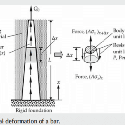
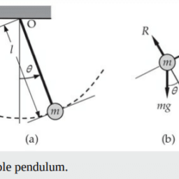
Consider the following pair of coupled differential equations governing bending of straight beams according to the Timoshenko beam theory, in which the normality condition (c) of the Euler-Bernoulli beam theory is removed:
$$
\begin{array}{r}
-\frac{d}{d x}\left[S\left(\frac{d w}{d x}+\phi\right)\right]+k w=q \
-\frac{d}{d x}\left(D \frac{d \phi}{d x}\right)+S\left(\frac{d w}{d x}+\phi\right)=0
\end{array}
$$
where $w$ is the transverse deflection, $\phi$ is the rotation of a transverse normal line, $S$ is the shear stiffness ( $S=K_s G A ; K_s$ is the shear correction coefficient, $G$ is the shear modulus, and $A$ is the area of cross section), $D=$ $E I$ is the bending stiffness, $k$ is the foundation modulus, and $q$ is the distributed transverse load. Develop the weak form of the above equations using the three-step procedure, identify the linear and bilinear forms, and determine the associated quadratic functional.
Solution: We use the three-step procedure to each of the two differential equations to develop the weak forms.
Multiply the first equation with weight function $v_1$ and the second equation with weight function $v_2$ and integrate over the length of the beam:
Step 1a
$$
0=\int_0^L v_1\left{-\frac{d}{d x}\left[S\left(\frac{d w}{d x}+\phi\right)\right]+k w-q\right} d x
$$
Step 2a
$$
\begin{aligned}
0= & \int_0^L\left[\frac{d v_1}{d x} S\left(\frac{d w}{d x}+\phi\right)+k v_1 w-v_1 q\right] d x-\left[v_1 S\left(\frac{d w}{d x}+\phi\right)\right]0^L \ = & \int_0^L\left[\frac{d v_1}{d x} S\left(\frac{d w}{d x}+\phi\right)+k v_1 w-v_1 q\right] d x-v_1(L)\left[S\left(\frac{d w}{d x}+\phi\right)\right]{x=L} \
& +v_1(0)\left[S\left(\frac{d w}{d x}+\phi\right)\right]{x=0} \end{aligned} $$ Step 1b $$ 0=\int_0^L v_2\left[-\frac{d}{d x}\left(D \frac{d \phi}{d x}\right)+S\left(\frac{d w}{d x}+\phi\right)\right] d x $$ Step 2b $$ \begin{aligned} 0 & =\int_0^L\left[D \frac{d v_2}{d x} \frac{d \phi}{d x}+v_2 S\left(\frac{d w}{d x}+\phi\right)\right] d x-\left[v_2 D \frac{d \phi}{d x}\right]_0^L \ & =\int_0^L\left[D \frac{d v_2}{d x} \frac{d \phi}{d x}+v_2 S\left(\frac{d w}{d x}+\phi\right)\right] d x-v_2(L)\left[D \frac{d \phi}{d x}\right]{x=L}+v_2(0)\left[D \frac{d \phi}{d x}\right]_{x=0}
\end{aligned}
$$
Note that integration by parts was used such that the expression $d w / d x+\phi$ is preserved, as it enters the boundary term representing the shear force. Such considerations can only be used by knowing the mechanics of the problem at hand. Also, note that the pair of weight functions $\left(v_1, v_2\right)$ satisfies the homogeneous form of specified essential boundary conditions on the pair $(w, \phi)$ (with the correspondence $v_1 \sim w$ and $\left.v_2 \sim \phi\right)$.
Consider the problem of determining the solution $u(x, y)$ to the partial differential equation
$$
-\frac{\partial}{\partial x}\left(a_{x x} \frac{\partial u}{\partial x}\right)-\frac{\partial}{\partial y}\left(a_{y y} \frac{\partial u}{\partial y}\right)+a_{00} u=f \text { in } \Omega
$$
in a closed two-dimensional domain $\Omega$ with boundary $\Gamma$, as shown in Fig. 2.2.4. Here $a_{00}, a_{x x}, a_{y y}$, and $f$ are known functions of position $(x, y)$ in $\Omega$. The function $u$ is required to satisfy, in addition to the differential equation (2.4.45), the following boundary conditions on the boundary $\Gamma$ of $\Omega$ :
$$
u=\hat{u} \text { on } \Gamma_u, a_{x x} \frac{\partial u}{\partial x} n_x+a_{y y} \frac{\partial u}{\partial y} n_y=\hat{q} \text { on } \Gamma_q
$$
where the portions $\Gamma_u$ and $\Gamma_q$ are such that $\Gamma=\Gamma_u \cup \Gamma_q$, as shown in Fig. 2.2.4. Develop the weak form, identify the linear and bilinear forms, and determine the quadratic functional for the problem.
Solution: The three-step procedure applied to Eq. (2.4.45) yields:
$$
\text { Step 1: } \quad \begin{aligned}
0= & \int_{\Omega} w\left[-\frac{\partial}{\partial x}\left(a_{x x} \frac{\partial u}{\partial x}\right)-\frac{\partial}{\partial y}\left(a_{y y} \frac{\partial u}{\partial y}\right)+a_{00} u-f\right] d x d y \
\text { Step 2: } \quad 0= & \int_{\Omega}\left(a_{x x} \frac{\partial w}{\partial x} \frac{\partial u}{\partial x}+a_{y y} \frac{\partial w}{\partial y} \frac{\partial u}{\partial y}+a_{00} w u-w f\right) d x d y \
& -\oint_{\Gamma} w\left(a_{x x} \frac{\partial u}{\partial x} n_x+a_{y y} \frac{\partial u}{\partial y} n_y\right) d s
\end{aligned}
$$
where we used integration by parts [see Eq. (2.2.43)] to transfer the differentiation from $u$ to $w$ so that both $u$ and $w$ have the same order derivatives. The boundary term shows that $u$ is the primary variable while
$$
a_{x x} \frac{\partial u}{\partial x} n_x+a_{y y} \frac{\partial u}{\partial y} n_y
$$
is the secondary variable.
Step 3: The last step in the procedure is to impose the specified boundary conditions in Eq. (2.4.46). Since $u$ is specified on $\Gamma_u$, then the weight function $w$ is zero on $\Gamma_u$ and arbitrary on $\Gamma_q$. Consequently, Eq. (2.4.47b) simplifies to
$$
0=\int_{\Omega}\left(a_{x x} \frac{\partial w}{\partial x} \frac{\partial u}{\partial x}+a_{y y} \frac{\partial w}{\partial y} \frac{\partial u}{\partial y}+a_{00} w u-w f\right) d x d y-\int_{\Gamma_q} w \hat{q} d s
$$
Variational Problem and Quadratic Functional: The weak form in Eq. (2.4.48) can be expressed as $B(w, u)=\ell(w)$, where the bilinear form and linear form are
$$
\begin{aligned}
B(w, u) & =\int_{\Omega}\left(a_{x x} \frac{\partial w}{\partial x} \frac{\partial u}{\partial x}+a_{y y} \frac{\partial w}{\partial y} \frac{\partial u}{\partial y}+a_{00} w u\right) d x d y \
\ell(w) & =\int_{\Omega} w f d x d y+\int_{\Gamma_q} w \hat{q} d s
\end{aligned}
$$
The associated quadratic functional is
$$
I(u)=\frac{1}{2} \int_{\Omega}\left[a_{x x}\left(\frac{\partial u}{\partial x}\right)^2+a_{y y}\left(\frac{\partial u}{\partial y}\right)^2+a_{00} u^2\right] d x d y-\int_{\Omega} u f d x d y-\int_{\Gamma_q} \hat{q} u d s
$$
In the case of transverse deflections of a membrane (with $a_{00}=0$ ), $I(u)$
Consider the differential equation
$$
-\frac{d^2 u}{d x^2}-u+x^2=0 \text { for } 0<x<1
$$
Determine $n$-parameter Ritz solutions using algebraic polynomials for the following two sets of boundary conditions:
Set 1: $u(0)=0, \quad u(1)=0$
Set 2: $u(0)=0,\left.\quad \frac{d u}{d x}\right|_{x=1}=1$
Numerically evaluate the solutions for $n=1,2$, and 3 .
Solution for Set 1 boundary conditions: The bilinear form and the linear functional associated with Eqs. (2.5.9) and (2.5.10) are
$$
B(w, u)=\int_0^1\left(\frac{d w}{d x} \frac{d u}{d x}-w u\right) d x, \quad \ell(w)=-\int_0^1 w x^2 d x
$$
Since both of the specified boundary conditions are of the essential type and homogeneous, we have $\phi_0=0$. The algebraic equations for this case are given by
$$
\begin{gathered}
\sum_{j=1}^n K_{i j} c_j=F_i, \quad i=1,2, \ldots, n \
K_{i j}=B\left(\phi_i, \phi_j\right)=\int_0^1\left(\frac{d \phi_i}{d x} \frac{d \phi_j}{d x}-\phi_i \phi_j\right) d x \
F_i=\ell\left(\phi_i\right)=-\int_0^1 \phi_i x^2 d x
\end{gathered}
$$
The same result as in Eqs. (2.5.13a) and (2.5.13b) can be obtained by minimizing the quadratic functional $I(u)$ in Eq. (2.4.26) [set $a=1, c=-1, f$ $=-x^2, L=1, Q_0=0$, and $\left.\beta=0\right]$ :
$$
I(u)=\frac{1}{2} \int_0^1\left[\left(\frac{d u}{d x}\right)^2-u^2+2 x^2 u\right] d x
$$
Substituting for $u \approx u_n$ from Eq. (2.5.4) with $\phi_0=0$ into the above functional, we obtain
$$
I\left(c_1, c_2, \ldots, c_n\right)=\frac{1}{2} \int_0^1\left[\left(\sum_{j=1}^n c_j \frac{d \phi_j}{d x}\right)^2-\left(\sum_{j=1}^n c_j \phi_j\right)^2+2 x^2\left(\sum_{j=1}^n c_j \phi_j\right)\right] d x
$$
The necessary condition for the minimum of $I$, which is a function of $n$ variables $c_1, c_2, \ldots, c_n$, is that its derivative with respect to each of the variables is zero:
$$
\begin{aligned}
\frac{\partial I}{\partial c_i}=0 & =\int_0^1\left[\frac{d \phi_i}{d x}\left(\sum_{j=1}^n c_j \frac{d \phi_j}{d x}\right)-\phi_i\left(\sum_{j=1}^n c_j \phi_j\right)+\phi_i x^2\right] d x \
0 & =\sum_{j=1}^n\left[\int_0^1\left(\frac{d \phi_i}{d x} \frac{d \phi_j}{d x}-\phi_i \phi_j\right) d x\right] c_j+\int_0^1 \phi_i x^2 d x \
& =\sum_{j=1}^n K_{i j} c_j-F_i \text { for } i=1,2, \ldots, n
\end{aligned}
$$
Clearly, Kij and Fi are the same as those defined in Eq. (2.5.13b).
Next we discuss the choice of $\phi_i$, which are required to satisfy the conditions $\phi_i(0)=\phi_i(1)=0$. Clearly, the polynomial $(0-x)(1-x)$ vanishes at $x=0$ and $x=1$, and its first derivative is nonzero. Hence, we take $\phi 1=x(1$ $-x)$. The next function in the sequence of complete functions is obviously $\phi_2=x_2(1-x)\left[\right.$ or $\left.\phi_2=x(1-x)^2\right]$. Thus, the following set of functions are admissible:
$$
\phi_1=x(1-x), \phi_2=x^2(1-x), \ldots, \phi_i=x^i(1-x), \ldots, \phi_n=x^n(1-x)
$$
The approximations

MY-ASSIGNMENTEXPERT™可以为您提供uq.edu MATH4604 Finite Element MethoD有限元方法的代写代考和辅导服务!