MY-ASSIGNMENTEXPERT™可以为您提供engineering MATH4604 Finite Element MethoD有限元方法的代写代考和辅导服务!
这是普渡大學有限元方法的代写成功案例。

CE595课程简介
• Academic integrity is expected of all students at all times. Further information on academic integrity policies may be found in the handbook University Regulations and on the Web at http://www.purdue.edu/ODOS/osrr/integrity.htm.
• Homework is due in class on the date indicated. In general, no late homework will be accepted. If you feel that you have serious extenuating circumstances (eg., illnesses or accidents requiring medical attention, personal or family crises), you must discuss your situation with Dr. Varma as soon as possible. In particular, foreseeable conflicts with due dates (eg., interviews, participation in sports activities, religious observances, etc.) must be brought to our attention before the due date.
• It is anticipated, even encouraged, that students will consult with each other on homework assignments. It is expected, however, that all work submitted by the student represent his/her own effort. Instances of plagiarism on an assignment will result in full loss of credit for that assignment.
• Instances of cheating in any form during an exam will result in full loss of credit for that exam. Additional measures, including immediate failure of the course, may be applied at the discretion of the instructor and/or University staff.
• Students who have documented disabilities and require accommodations must make an appointment with Dr. Varma to discuss their needs by the end of the second week of class. Students with disabilities must be registered with Adaptive Programs in the Office of the Dean of Students before classroom accommodations can be provided.
Prerequisites
Grades will be based upon the following elements:
• Homework (25% of total grade) Due in class at dates to be announced.
• Hourly Exam #1 (25% of total grade) Tentatively scheduled for February last week.
• Hourly Exam #2 (25% of total grade) Tentatively scheduled for April first week.
• Course Project or Final Exam (25% of total grade) Schedule will be announced later in the semester.
CE595 Finite Element Method HELP(EXAM HELP, ONLINE TUTOR)
Problem statement: Consider the problem of determining the perimeter (a quantity of interest) of a circle of radius $R$, as shown in Fig. 1.4.3(a). Pretend that we do not know the formula $(P=2 \pi R)$ for the perimeter $P$ (circumference) of a circle. Babylonians estimated the value of the perimeter of a circle by approximating it by straight line segments, whose lengths they were able to measure. Obtain the approximate value of the circumference by representing it as a sum of the lengths of the line segments.
Solution: The three basic features of the finite element method in the present case take the following form. First, the division of the perimeter of a circle into a collection of line segments. In theory, we need infinite number of such line elements to represent the perimeter; otherwise, the value computed will have some error. Second, writing an equation for the quantity of interest (perimeter) over an element (line segment) in this case is exact, because the approximated perimeter is a straight line. Third, the assembly of elements amounts to simply adding the element lengths to obtain the total value. Although this is a trivial example, it illustrates several (but not all) ideas and steps involved in the finite element analysis of a problem. We outline the steps involved in computing an approximate value of the perimeter of the circle. In doing so, we introduce certain terms that are used in the finite element analysis of any problem.
Finite element discretization. First, the domain (i.e., the perimeter of the circle) is represented as a collection of a finite number $n$ of subdomains, namely, line segments, as shown in Fig. 1.4.3(b). This is called discretization of the domain. Each subdomain (i.e., line segment) is called an element. The collection of elements is called the finite element mesh. The elements are connected to each other at points called nodes. In the present case, we discretize the perimeter into a mesh of five $(n=5)$ line segments, as shown in Fig. 1.4.3(c).
The line segments can be of different lengths. When all elements are of the same length, the mesh is said to be uniform; otherwise, it is called a nonuniform mesl.
Element equations. A typical element (i.e., line segment, $\Omega_e$ ) is isolated and its required properties, i.e., length, are computed by some appropriate means. Let $h_e$ be the length of element $\Omega_e$ in the mesh. For a typical element $\Omega_e, h_c$ is given, as can be seen from $\Gamma$ ig. 1.4.3(d), by
$$
h_e=2 R \sin \frac{1}{2} \theta_e
$$
where $R$ is the radius of the circle and $\theta_e<u$ is the angle subtended by the line segment. The above equations are called element equations. Ancient mathematicians most likely made measurements, rather than using Eq. (1.4.1), to find $h_e$ (they did not know $\pi$ ).
Assembly of element equations and solution. The approximate value of the perimeter of the circle is obtained by putting together the element properties in a meaning[ul way; this process is called the assembly of the element equations. It is based, in the present case, on the simple idea that the total perimeter of the polygon $\Omega_h$ (assembly of elements) is equal to the sum of the lengths of individual elements:
$$
P_n=\sum_{e=1}^n h_e
$$
Then $P_n$ represents an approximation to the actual perimeter, $P$. If the mesh is uniform, or $h_e$ is the same for each of the elements in the mesh, then $\theta_e=2 \pi / n$, and we have
$$
P_n=n\left(2 R \sin \frac{\pi}{n}\right)
$$
Convergence and error estimate. For this simple problem, we know the exact solution: $P=2 \pi R$. We can estimate the error in the approximation and show that the approximate solution $P_n$ converges to the exact value $P$ in the limil as $n \rightarrow \infty$. Consider a typical element $\Omega_e$. The error in the approximation is equal to the difference between the length of the sector and that of the line segment [see Fig. 1.4.3(d)]
$$
E_e=\left|S_e-h_e\right|
$$
where $S_e=R \theta_e$ is the length of the sector. Thus, the error estimate for an element in the mesh is given by
$$
E_e=R\left(\frac{2 \pi}{n}-2 \sin \frac{\pi}{n}\right)
$$
The total error (called global error) is given by multiplying $E_e$ by $n$ :
$$
E=n E_e=2 R\left(\pi-n \sin \frac{\pi}{n}\right)=2 \pi R-P_n=P-P_n
$$
We now show that $E$ goes to zero as $n \rightarrow \infty$. Letting $x=1 / n$, we have
$$
P_n=2 R n \sin \frac{\pi}{n}=2 R \frac{\sin \pi x}{x}
$$
and
$$
\lim {n \rightarrow \infty} P_n=\lim {x \rightarrow 0}\left(2 R \frac{\sin \pi x}{x}\right)=\lim _{x \rightarrow 0}\left(2 \pi R \frac{\cos \pi x}{1}\right)=2 \pi R
$$
Hence, $E_n$ goes to zero as $n \rightarrow \infty$. This completes the proof of convergence.
Compute the determinant and inverse of the matrix
$$
\mathbf{A}=\left[\begin{array}{rrr}
2 & 5 & -1 \
1 & 4 & 3 \
2 & -3 & 5
\end{array}\right]
$$
Solution: The minors are
$$
\begin{array}{lll}
M_{11}(\mathbf{A})=\left|\begin{array}{rr}
4 & 3 \
-3 & 5
\end{array}\right|, & M_{12}(\mathbf{A})=\left|\begin{array}{rr}
1 & 3 \
2 & 5
\end{array}\right|, & M_{13}(\mathbf{A})=\left|\begin{array}{rr}
1 & 4 \
2 & -3
\end{array}\right| \
M_{21}(\mathbf{A})=\left|\begin{array}{rr}
5 & -1 \
-3 & 5
\end{array}\right|, & M_{22}(\mathbf{A})=\left|\begin{array}{rr}
2 & -1 \
2 & 5
\end{array}\right|, & M_{23}(\mathbf{A})=\left|\begin{array}{rr}
2 & 5 \
2 & -3
\end{array}\right| \
M_{31}(\mathbf{A})=\left|\begin{array}{rr}
5 & -1 \
4 & 3
\end{array}\right|, & M_{32}(\mathbf{A})=\left|\begin{array}{rr}
2 & -1 \
1 & 3
\end{array}\right|, & M_{33}(\mathbf{A})=\left|\begin{array}{ll}
2 & 5 \
1 & 4
\end{array}\right|
\end{array}
$$
To compute the determinant, we use the definition in Eq. (2.2.48) and expand by the first column and obtain
$$
\begin{aligned}
|A| & =\sum_{i=1}^3(-1)^{i+1} a_{i 1}\left|A_{i 1}\right|=a_{11} M_{11}(\mathbf{A})-a_{21} M_{21}(\mathbf{A})+a_{31} M_{31}(\mathbf{A}) \
& =a_{11}\left|\begin{array}{rr}
4 & 3 \
-3 & 5
\end{array}\right|-a_{21}\left|\begin{array}{rr}
5 & -1 \
-3 & 5
\end{array}\right|+a_{31}\left|\begin{array}{rr}
5 & -1 \
4 & 3
\end{array}\right| \
& =2[(4)(5)-(3)(-3)]+(-1)[(5)(5)-(-1)(-3)]+2[(5)(3)-(-1)(4)] \
& =2(20+9)-(25-3)+2(15+4)=74
\end{aligned}
$$
We note that the determinant also can be computed by expanding by the first row:
$$
\begin{gathered}
|A|=a_{11} M_{11}(\mathbf{A})-a_{12} M_{12}(\mathbf{A})+a_{13} M_{13}(\mathbf{A})=2 \times 29-5 \times(-1)+(-1) \times \
(-11)=74
\end{gathered}
$$
To compute the inverse of the given matrix we first compute the cofactors:
$$
\begin{aligned}
& \operatorname{cof}{11}(\mathbf{A})=(-1)^2 M{11}(\mathbf{A})=4 \times 5-(-3) 3=29 \
& \operatorname{cof}{12}(\mathbf{A})=(-1)^3 M{12}(\mathbf{A})=-(1 \times 5-3 \times 2)=1 \
& \operatorname{cof}{13}(\mathbf{A})=(-1)^4 M{13}(\mathbf{A})=1 \times(-3)-2 \times 4=-11 \
& \operatorname{cof}{21}(\mathbf{A})=(-1)^3 M{21}(\mathbf{A})=-[5 \times 5-(-3)(-1)]=-22 \
& \operatorname{cof}{22}(\mathbf{A})=(-1)^4 M{22}(\mathbf{A})=[2 \times 5-2 \times(-1)]=12 \
& \operatorname{cof}{23}(\mathbf{A})=(-1)^5 M{23}(\mathbf{A})=-[2 \times(-3)-2 \times 5]=16
\end{aligned}
$$
and so on. Then the Adj (A) is given by cof11 (A) cof12 (A) cof13 (A)
$$
\operatorname{Adj}(\mathbf{A})=\left[\begin{array}{lll}
\operatorname{cof}{11}(\mathbf{A}) & \operatorname{cof}{12}(\mathbf{A}) & \operatorname{cof}{13}(\mathbf{A}) \ \operatorname{cof}{21}(\mathbf{A}) & \operatorname{cof}{22}(\mathbf{A}) & \operatorname{cof}{23}(\mathbf{A}) \
\operatorname{cof}{31}(\mathbf{A}) & \operatorname{cof}{32}(\mathbf{A}) & \operatorname{cof}_{33}(\mathbf{A})
\end{array}\right]^{\mathrm{T}}=\left[\begin{array}{rrr}
29 & -22 & 19 \
1 & 12 & -7 \
-11 & 16 & 3
\end{array}\right]
$$
The inverse of $\mathbf{A}$ can be now computed using Eq. (2.2.51):
$$
\mathbf{A}^{-1}=\frac{1}{74}\left[\begin{array}{rrr}
29 & -22 & 19 \
1 & 12 & -7 \
-11 & 16 & 3
\end{array}\right]
$$
It can be easily verified that $\mathbf{A A}^{-1}=\mathbf{A}^{-1} \mathbf{A}=\mathbf{I}$.
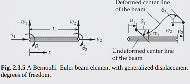
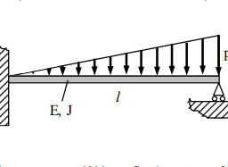
Determine the strain energy density $U_0$ and strain energy of a BernoulliEuler beam of length $L$, area of cross section $A$, moment of inertia $I$, and modulus $E$. Assume that the material of the beam is linearly elastic, deformation is infinitesimal, and the displacement components at any point $(x, y, z)$ in the beam can be expressed in terms of the two unknown $(u, w)$ as follows:
$$
u_1=u(x)-z \frac{d w}{d x} \quad u_2=0, u_3=w(x)
$$
Note that the beam is stretched and bent by external forces in the $x z$-plane only.
Solution: The only nonzero linear strain is
$$
\varepsilon_{x x}=\frac{d u}{d x}-z \frac{d^2 w}{d x^2}
$$
The strain energy density is
$$
\begin{aligned}
U_0 & =\int_0^{\varepsilon_{x x}} \sigma_{x x} d \varepsilon_{x x}=\int_0^{\varepsilon_{x x}} E \varepsilon_{x x} d \varepsilon_{x x} \
& =\frac{E}{2} \varepsilon_{x x}^2=\frac{E}{2}\left(\frac{d u}{d x}-z \frac{d^2 w}{d x^2}\right)^2
\end{aligned}
$$
The strain energy $U$ is given by
$$
\begin{aligned}
U & =\int_{\Omega} U_0 d \Omega=\int_0^L \int_A \frac{E}{2}\left(\frac{d u}{d x}-z \frac{d^2 w}{d x^2}\right)^2 d A d x \
& =\frac{1}{2} \int_0^L\left[A_{x x}\left(\frac{d u}{d x}\right)^2+D_{x x}\left(\frac{d^2 w}{d x^2}\right)^2\right] d x
\end{aligned}
$$
where $A_{x x}$ and $D_{x x}$ are defined as (for the case in which $E$ is at most a function of $x$ )
$$
A_{x x}=\int_A E d A=E A, \quad D_{x x}=\int_A z^2 E d A=E I
$$
we have
$$
U=\frac{1}{2} \int_0^L\left[E A\left(\frac{d u}{d x}\right)^2+E I\left(\frac{d^2 w}{d x^2}\right)^2\right] d x
$$
where we have used the fact (because $x$-axis is taken along the geometric centroid)
$$
\int_A z d A=0
$$

MY-ASSIGNMENTEXPERT™可以为您提供ENGINEERING MATH4604 FINITE ELEMENT METHOD有限元方法的代写代考和辅导服务!