MY-ASSIGNMENTEXPERT™可以为您提供engineering MATH4604 Finite Element MethoD有限元方法的代写代考和辅导服务!
这是普渡大學有限元方法的代写成功案例。
CE595课程简介
• Academic integrity is expected of all students at all times. Further information on academic integrity policies may be found in the handbook University Regulations and on the Web at http://www.purdue.edu/ODOS/osrr/integrity.htm.
• Homework is due in class on the date indicated. In general, no late homework will be accepted. If you feel that you have serious extenuating circumstances (eg., illnesses or accidents requiring medical attention, personal or family crises), you must discuss your situation with Dr. Varma as soon as possible. In particular, foreseeable conflicts with due dates (eg., interviews, participation in sports activities, religious observances, etc.) must be brought to our attention before the due date.
• It is anticipated, even encouraged, that students will consult with each other on homework assignments. It is expected, however, that all work submitted by the student represent his/her own effort. Instances of plagiarism on an assignment will result in full loss of credit for that assignment.
• Instances of cheating in any form during an exam will result in full loss of credit for that exam. Additional measures, including immediate failure of the course, may be applied at the discretion of the instructor and/or University staff.
• Students who have documented disabilities and require accommodations must make an appointment with Dr. Varma to discuss their needs by the end of the second week of class. Students with disabilities must be registered with Adaptive Programs in the Office of the Dean of Students before classroom accommodations can be provided.
Prerequisites
Grades will be based upon the following elements:
• Homework (25% of total grade) Due in class at dates to be announced.
• Hourly Exam #1 (25% of total grade) Tentatively scheduled for February last week.
• Hourly Exam #2 (25% of total grade) Tentatively scheduled for April first week.
• Course Project or Final Exam (25% of total grade) Schedule will be announced later in the semester.
CE595 Finite Element Method HELP(EXAM HELP, ONLINE TUTOR)
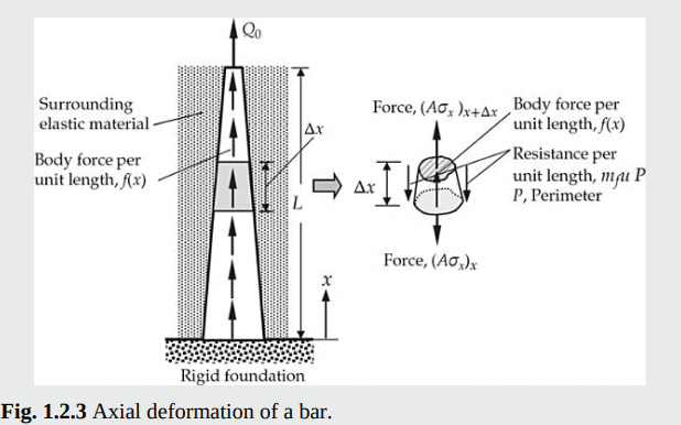
Problem statement (Deformation of a bar embedded in a matrix material): Consider a pile embedded in an elastic material and subjected to an axial force $Q_0$. The resistance offered by the surrounding material to the movement of the bar is assumed to be linearly proportional to the displacement, $u$. Thus, the force per unit surface area of the rod is $m_j u$, where $m_j$, represents the proportionality parameter. The weight of the body, $f(x)$ measured per unit length, is assumed to be negligible compared to the applied load $Q_0$, but include it in the derivation for generality. Derive the governing equation of the problem.
Solution: First, we know that the significant load taken by a pile is vertical. So the axial deformation and stress will be the significant quantities, and the lateral deformation due to the Poisson effect may be neglected. Second, we wish to consider the static case. The governing equations of this simplified problem can be obtained using Newton’s second law and a uniaxial stressstrain (constitutive) relation for the material of the bar. The reader should note the similarity in the derivation of the equations of this solid mechanics problem with the heat flow problem discussed earlier.
Figure 1.2.3 shows an element of length $\Delta x$ with axial forces acting at both ends of the element, where $\sigma_x$ denotes stress i.e., force per unit area; $\mathrm{N} / \mathrm{m}^2$ in the $x$ direction, which is taken positive upward; $f(x)$ denotes the body force measured per unit length $(\mathrm{N} / \mathrm{m})$. Hence, $\left[A \sigma_x\right]x$ is the net tensile force on the volume element at $x$ and $\left[A \sigma_x\right]{x+\Delta x}$ is the net tensile force at $x+$ $\Delta x$. The resistance of the surrounding medium is $m_j u P$ per unit length in the direction opposite to the force $Q_0$, where $P$ is the perimeter. Then setting the sum of the forces to zero i.e., applying Newton’s second law in the $x$ direction yields
$$
-\left[A \sigma_x\right]x+\left[A \sigma_x\right]{x+\Delta x}+f \Delta x-m_f u P \Delta x=0
$$
Dividing throughout by $\Delta x$ and taking the limit $\Delta x \rightarrow 0$, we obtain
$$
\frac{d}{d x}\left(A \sigma_x\right)-c u+f(x)=0
$$
where $c=m_j P$.
The stress $\sigma_x$ can be related to the axial displacement using Hooke’s law and straindisplacement relation
$$
\sigma_x=E \varepsilon_x, \quad \varepsilon_x=\frac{d u}{d x}
$$
where $E$ is Young’s modulus $\left.\mathrm{N} / \mathrm{m}^2\right), u(x)$ denotes the axial displacement $(\mathrm{m})$ and $\varepsilon_x$ is the axial strain $(\mathrm{m} / \mathrm{m}$. Again, Eq. (1.2.25) represents a constitutive equation. Note that a system can have several constitutive relations, each depending on the phenomenon being studied. The study of heat transfer in a bar required us to employ Fourier’s law to relate temperature gradient to heat flux, and the study of deformation of the same bar subjected to axial forces requires us to use Hooke’s law to connect stress to displacement gradient.
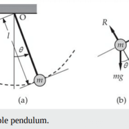
Problem statement (The pendulum problem): Consider Eq. (1.2.4) governing the simple planar motion of a pendulum subject to the initial conditions in Eq. (1.2.5). Use the forward and backward finite difference methods to formulate discretized forms of the equation. Obtain numerical solutions for three different time steps, $\Delta t=0.05, \Delta t=0.025$, and $\Delta t=0.001$, and compare them graphically with the exact linear solution. Take $\ell=2.0, g=$ 32.2, $\theta_0=\pi / 4$, and $v_0=0$ in the numerical computation.
Solution: We begin with the following general first-order differential equation [of which Eq. (1.2.4) is a special case]
$$
\frac{d u}{d t}=f(t, u), \quad 00$ subject to the initial (i.e., time $t=0$ ) condition $u(0)=u_0$. We approximate the derivative at time $t=t_i$ by
$$
\left.\left(\frac{d u}{d t}\right)\right|{t=t_i} \approx \frac{u\left(t{i+1}\right)-u\left(t_i\right)}{t_{i+1}-t_i}
$$
We note that the derivative at $t=t_i$ is replaced by its definition except that we did not take the limit $\Delta t \equiv t_{i+1}-t_i \rightarrow 0$; that is why it is an approximation. We also note that the slope of $u$ at $t_i$ in Eq. (1.3.2) is based on values of $u$ at $t_i$ and $t_{i+1}$. We can also take it to be the slope at $t=t_{i+1}$
$$
\left.\left(\frac{d u}{d t}\right)\right|{t=t{i+1}} \approx \frac{u\left(t_{i+1}\right)-u\left(t_i\right)}{t_{i+1}-t_i}
$$
The formula in Eq. (1.3.2) is called, for obvious reasons, forward difference, while that in Eq. (1.3.3) is called backward difference. The forward difference scheme is also known as Euler’s explicit scheme or first-order Runge-Kutta method. For increasingly small values of $\Delta t$, we hope that both approximations have a decreasingly small error in the computation of the slope. However, the two schemes will have different numerical convergence and stability behavior, as will be discussed in more detail in Chapter 7.
Substituting Eq. (1.3.2) into Eq. (1.3.1) at $t=t_i$, we obtain the forward difference formula
$$
u_{i+1}=u_i+\Delta t f\left(u_i, t_i\right), \quad u_i=u\left(t_i\right), \Delta t=t_{i+1}-t_i
$$
Equation (1.3.4) can be solved, starting from the known value $u_0$ of $u(t)$ at $t$ $=0$, for $u_1=u\left(t_1\right)=u(\Delta t)$. This process can be repeated to determine the values of $u$ at times $t=\Delta t, 2 \Delta t, \ldots, n \Delta t$. Of course, there are higher-order finite difference schemes that are more accurate than the Euler’s scheme and we will not discuss them as they are outside the scope of this study. Note that we are able to convert the ordinary differential equation, Eq. (1.3.1), to an algebraic equation, Eq. (1.3.4), which needs to be evaluated at different times to construct the time history of $u(t)$.
Problem statement (The heat flow problem): Consider the boundary-value problem of Example 1.2.2. Use the centered difference method to determine the numerical solution of Eq. (1.2.19):
$$
-\frac{d^2 \theta}{d x^2}+m^2 \theta=0, m=\sqrt{\frac{\beta P}{k A}}, 0<x<L
$$
Solution: First we divide the domain $(0, L)$ into a finite set of $N$ intervals of equal length $\Delta x$, as shown in Fig. 1.3.2(b). Then we approximate the second derivative of $\theta=T-T_{\infty}$ directly using the centered difference scheme [error is of order $O(\Delta x)^2$ ] $\left(\frac{d^2 \theta}{d x^2}\right){x=x_i} \approx\left(\frac{\theta{i-1}-2 \theta_i+\theta_{i+1}}{(\Delta x)^2}\right)$
This approximation involves three points, called mesh points, at which function evaluations are required. The mesh points are separated by a distance of $\Delta x$. Using the above approximation in Eq. (1.2.19), we obtain
$$
-\left(\theta_{i-1}-2 \theta_i+\theta_{i+1}\right)+(m \Delta x)^2 \theta_i=0 \text { or }-\theta_{i-1}+\left[2+(m \Delta x)^2\right] \theta_i-\theta_{i+1}=0
$$
Equation (1.3.8) is valid for any mesh point $x=x_i, i=1,2, \ldots, N$, at which the solution is not known. The formula contains values of $\theta$ at three mesh points $x=x_{i-1}, x_i$, and $x=x_{i+1}$ at a time. Note that Eq. (1.3.8) is not used at mesh point $x=x_0=0$ because the temperature is known there, as given in Eq. (1.2.20). However, use of Eq. (1.3.8) at mesh point $x=x_N=L$ requires the knowledge of the fictitious value $\theta_{N+1}$ (as we see in the sequel, we never have to deal with such fictitious values in the finite element method). The forward finite difference approximation of the second boundary condition in Eq. (1.2.20) at mesh point $x_N=L$ can be used to determine $\theta_{N+1}$ :
$$
\frac{\theta_{N+1}-\theta_N}{\Delta x}+\frac{\beta}{k} \theta_N=0 \Rightarrow \theta_{N+1}=\left(1-\frac{\beta \Delta x}{k}\right) \theta_N
$$
Application of the formula in Eq. (1.3.7) to mesh points at $x_1, x_2, \ldots, x_N$ yields
$$
\begin{array}{r}
-\theta_0+D \theta_1-\theta_2=0 \
-\theta_1+D \theta_2-\theta_3=0 \
-\theta_2+D \theta_3-\theta_4=0 \
\cdots \quad \cdots \quad \cdots \
-\theta_{N-1}+D \theta_N-\theta_{N+1}=0
\end{array}
$$
where $D=\left[2+(m \Delta x)^2\right]$. Equation (1.3.9) can be used to eliminate $\theta_{N+1}$ from the last equation in (1.3.10). Then Eq. (1.3.10) consists of $N$ equations in $N$ unknowns, $\theta_1, \theta_2, \ldots, \theta_N$.

MY-ASSIGNMENTEXPERT™可以为您提供ENGINEERING MATH4604 FINITE ELEMENT METHOD有限元方法的代写代考和辅导服务!