物理代写| PlaneWave Solutions 相对论代考
物理代写
8.4 Plane Wave Solutions
We consider the simplest type of solutions and also the most important type of solutions, namely, the plane wave solutions-the surfaces of constant phase are planes or more precisely, hyperplanes in the background four dimensional Minkowski space. Astrophysically, since the sources are at a very large distance from the detectors, the waves would be plane to a great degree of accuracy.
We set the right hand side in Eq. (8.2.10), namely, the source term to zero, and so we have the equation:
$$
\square \bar{h}{\mu \nu}=0 . $$ We now consider solutions of the form, $$ \bar{h}{\mu v}=A_{\mu v} e^{-i k_{\alpha} x^{\alpha}}
$$
where $A_{\mu \nu}$ is a constant symmetric matrix and $k_{\alpha}$ is a constant vector called the wave vector and signifies the direction of the wave in the 4 dimensional spacetime. Substituting this solution in the wave equation gives:
$$
\begin{aligned}
\square \bar{h}^{\mu v}=\eta^{\alpha \beta} \bar{h}{, \alpha \beta}^{\mu v} &=-\eta^{\alpha \beta} k{\alpha} k_{\beta} \bar{h}^{\mu v} \equiv 0 \
& \Longrightarrow \eta^{\alpha \beta} k_{\alpha} k_{\beta}=0
\end{aligned}
$$
Or $k_{\alpha} k^{\alpha}=0$, which implies that the wave vector $k^{\alpha}$ is null. Thus, GW waves travel with the speed $c$ which is also the speed of light. This is the first result of GR.
We will further also show that the waves are transverse. The Lorenz gauge condition Eq. (8.2.5) gives,
Thus GW are transverse.
8 Gravitational Waves
136
8.4.1 The Transverse Traceless (TT) Gauge because we can still remain within the Lorenz gauge by further choosing $\xi^{\mu}$ such that $\square \xi^{\mu}=0$ (instead of using $\zeta^{\mu}$ we persist with $\xi^{\mu}$ without any cause for confusion). Let us choose $\xi_{\mu}=B_{\mu} e^{-i k_{\alpha} x^{\alpha}}$ then, Eq. (8.3.5) gives,
$$
A_{\mu \nu}^{\prime}=A_{\mu \nu}+i B_{\mu} k_{v}+i B_{\nu} k_{\mu}-i \eta_{\mu \nu} B^{\alpha} k_{\alpha} .
$$
We see that we automatically remain in the Lorenz guage because,
$$
A_{\mu \nu}^{\prime} k^{\nu}=A_{\mu \nu} k^{\nu}+i B_{\mu} k_{\nu} k^{\nu}+i B_{v} k^{v} k_{\mu}-i \eta_{\mu \nu} k^{v} B^{\alpha} k_{\alpha} \equiv 0
$$
because first two terms on the RHS of Eq. (8.4.6) are zero and the last two terms cancel out. This is no surprise because we are within the Lorenz gauges.
The additional gauge freedom allows us to make $A_{\mu v}$ tracefree, that is,
$$
A_{\mu}^{\mu}=0
$$
and further for any given timelike vector $U^{\mu}$ we are allowed to choose:
$$
A_{\mu \nu} U^{\nu}=0 .
$$
The equations (8.4.7) and (8.4.8) can be easily shown to hold in the new guage by explicitly solving for $B_{\mu}$ in terms of the old $A_{\mu \nu}$. See Exercise 8.1.
Since $A_{\mu \nu}$ can be considered as a symmetric matrix, it has at most 10 independent components. The Lorenz gauge condition $A_{\mu v} k^{\nu}=0$, Eqs. (8.4.7) and (8.4.8) constitute 8 independent conditions on these 10 components of $A_{\mu v}$. Therefore, $A_{\mu v}$ has only 2 independent components and these are the physical degrees of freedom of the GW-the two polarisations. The above conditions fix the gauge and is called the transverse traceless gauge or the TT gauge for short. The $A_{\mu \nu}$ matrix is denoted by $A_{\mu \nu}^{T T}$ in this gauge and the corresponding $h_{\mu \nu}$ by $h_{\mu \nu}^{T T}$.
8.4 Plane Wave Solutions
137
$$
A_{\mu v}^{T T}=\left(\begin{array}{rrrr}
0 & 0 & 0 & 0 \
0 & A_{x x} & A_{x y} & 0 \
0 & A_{x y} & -A_{x x} & 0 \
0 & 0 & 0 & 0
\end{array}\right)
$$
It is customary to write $A_{x x}=A_{+}$and $A_{x y}=A_{\times}$for reasons that will become clear later in the text. We therefore write $A_{x x}=A_{+}$and $A_{x y}=A_{\times}$and the corresponding $h_{+}=A_{+} e^{-i k_{\alpha} x^{\alpha}}$ and $h_{\times}=A_{\times} e^{-i k_{\alpha} x^{\alpha}} .$ We can associate polarisation tensors corresponding to each polarisation (just as there are polarisation vectors for the electromagnetic wave):
$$
e_{\mu v}^{+}=\left(\begin{array}{rrrr}
0 & 0 & 0 & 0 \
0 & 1 & 0 & 0 \
0 & 0 & -1 & 0 \
0 & 0 & 0 & 0
\end{array}\right), \quad e_{\mu v}^{\times}=\left(\begin{array}{llll}
0 & 0 & 0 & 0 \
0 & 0 & 1 & 0 \
0 & 1 & 0 & 0 \
0 & 0 & 0 & 0
\end{array}\right)
$$
These are the plus $(+)$ and cross $(x)$ polarisation tensors. Each of the polarisation tensors describe linear polarisation again denoted by $+$ and $\times$. The nomenclature will become clear in the next section when we consider the effect of each polarisation separately on a ring of test particles. The general wave is a linear combination of the two polarisations and can be written in terms of the polarisation tensors:
$$
h_{\mu v}^{T T}=h_{+} e_{\mu v}^{+}+h_{\times} e_{\mu v}^{\times} .
$$
Here we have polarisation tensors because we have a tensor wave. The polarisations can have a phase difference between them which is realised by the fact that the $A_{+}$ and $A_{\times}$can be complex quantities and so the phases are be accommodated in the phases of the complex numbers.
The polarisation tensors are orthogonal in the sense that their scalar product is zero:
$$
e_{\mu v}^{+} e^{\times \mu v}=0
$$
In the above discussion we have restricted ourselves to a specific frequency $\omega$ of the wave. These results can be easily generalised to a wave coming from a fixed direction, as a general function of $t$. The result follows on taking the inverse Fourier transform with respect to $\omega$. Then the GW amplitudes $h_{+, \times}$become functions of $t$, that is, now we have $h_{+}(t), h_{\times}(t), h_{\mu \nu}^{T T}(t)$ etc. Much of the above discussion follows (Schutz 1995). For further reading we refer the reader to Misner et al. (1973) and Schutz (1995).

物理代考
8.4 平面波解决方案
我们考虑最简单的解类型,也是最重要的解类型,即平面波解——恒定相位的表面是平面,或者更准确地说,是背景四维 Minkowski 空间中的超平面。在天体物理学上,由于源与探测器的距离非常大,因此波会在很大程度上是平面的。
我们在等式中设置右手边。 (8.2.10),即源项为零,所以我们有等式:
$$
\square \bar{h}{\mu \nu}=0 。 $$ 我们现在考虑以下形式的解决方案, $$ \bar{h}{\mu v}=A_{\mu v} e^{-i k_{\alpha} x^{\alpha}}
$$
其中 $A_{\mu \nu}$ 是一个常数对称矩阵,$k_{\alpha}$ 是一个常数向量,称为波向量,表示波在 4 维时空中的方向。将此解代入波动方程得到:
$$
\开始{对齐}
\square \bar{h}^{\mu v}=\eta^{\alpha \beta} \bar{h}{, \alpha \beta}^{\mu v} &=-\eta^{\阿尔法 \beta} k{\alpha} k_{\beta} \bar{h}^{\mu v} \equiv 0 \
& \Longrightarrow \eta^{\alpha \beta} k_{\alpha} k_{\beta}=0
\end{对齐}
$$
或$k_{\alpha} k^{\alpha}=0$,这意味着波向量$k^{\alpha}$ 为空。因此,GW 波以 $c$ 的速度传播,这也是光速。这是GR的第一个结果。
我们还将进一步证明波是横向的。洛伦兹规范条件方程。 (8.2.5) 给出,
因此GW是横向的。
8 引力波
136
8.4.1 横向无迹(TT)规范,因为我们仍然可以通过进一步选择 $\xi^{\mu}$ 使得 $\square \xi^{\mu}=0$(而不是使用$\zeta^{\mu}$ 我们坚持使用 $\xi^{\mu}$ 没有任何混淆)。让我们选择 $\xi_{\mu}=B_{\mu} e^{-i k_{\alpha} x^{\alpha}}$ 然后,等式。 (8.3.5) 给出,
$$
A_{\mu \nu}^{\prime}=A_{\mu \nu}+i B_{\mu} k_{v}+i B_{\nu} k_{\mu}-i \eta_{\mu \nu} B^{\alpha} k_{\alpha} 。
$$
我们看到我们自动保持在 Lorenz 量表中,因为,
$$
A_{\mu \nu}^{\prime} k^{\nu}=A_{\mu \nu} k^{\nu}+i B_{\mu} k_{\nu} k^{\nu} +i B_{v} k^{v} k_{\mu}-i \eta_{\mu \nu} k^{v} B^{\alpha} k_{\alpha} \equiv 0
$$
因为方程式 RHS 的前两项。 (8.4.6) 为零,最后两项抵消。这并不奇怪,因为我们在 Lorenz 量规范围内。
额外的规范自由度允许我们使 $A_{\mu v}$ 无迹,即
$$
A_{\mu}^{\mu}=0
$$
并且进一步对于任何给定的类时向量 $U^{\mu}$ 我们可以选择:
$$
A_{\mu \nu} U^{\nu}=0 。
$$
通过根据旧的 $A_{\mu \nu}$ 显式求解 $B_{\mu}$,可以很容易地证明方程 (8.4.7) 和 (8.4.8) 在新量规中成立。见练习 8.1。
由于 $A_{\mu \nu}$ 可以被认为是一个对称矩阵,它最多有 10 个独立分量。洛伦兹规范条件 $A_{\mu v} k^{\nu}=0$,方程。 (8.4.7) 和 (8.4.8) 在 $A_{\mu v}$ 的这 10 个分量上构成 8 个独立条件。因此,$A_{\mu v}$ 只有 2 个独立分量,它们是 GW 的物理自由度——两个极化。以上条件固定量规,简称横向无痕量规或TT量规。 $A_{\mu \nu}$ 矩阵在这个规范中用 $A_{\mu \nu}^{TT}$ 表示,对应的 $h_{\mu \nu}$ 用 $h_{\mu \nu }^{TT}$。
8.4 平面波解决方案
137
$$
A_{\mu v}^{T T}=\left(\begin{array}{rrrr}
0 & 0 & 0 & 0 \
0 & A_{x x} & A_{x y} & 0 \
0 & A_{x y} & -A_{x x} & 0 \
0 & 0 & 0 & 0
\end{数组}\右)
$$
习惯上写成 $A_{x x}=A_{+}$ 和 $A_{x y}=A_{\times}$,原因将在下文中变得清楚。因此我们写成 $A_{xx}=A_{+}$and $A_{xy}=A_{\times}$ 和对应的 $h_{+}=A_{+} e^{-i k_{\alpha} x^{\alpha}}$ 和 $h_{\times}=A_{\times} e^{-i k_{\alpha} x^{\alpha}} .$ 我们可以关联每个极化对应的极化张量 (就像电磁波有极化矢量一样):
$$
e_{\mu v}^{+}=\left(\begin{array}{rrrr}
0 & 0 & 0 & 0 \
0 & 1 & 0 & 0 \
0 & 0 & -1 & 0 \
0 & 0 & 0 & 0
\end{array}\right), \quad e_{\mu v}^{\times}=\left(\begin{array}{llll}
0 & 0 & 0 & 0 \
0 & 0 & 1 & 0 \
0 & 1 & 0 & 0 \
0 & 0 & 0 & 0
\end{数组}\右)
$$
这些是加 $(+)$ 和交叉 $(x)$ 极化张量。每个极化张量都描述了线性极化,再次用 $+$ 和 $\times$ 表示。当我们分别考虑每个极化对测试粒子环的影响时,命名将在下一节中变得清晰。一般波是两个极化的线性组合,可以用极化张量写成:
$$
h_{\mu v}^{T T}=h_{+} e_{\mu v}^{+}+h_{\times} e_{\mu v}^{\times} 。
$$
这里我们有极化张量,因为我们有张量波。极化可以在它们之间有相位差,这是通过 $A_{+}$ 和 $A_{\times}$ 可以是复数的事实来实现的,因此相位可以容纳在 comp

物理代考Gravity and Curvature of Space-Time 代写 请认准UprivateTA™. UprivateTA™为您的留学生涯保驾护航。
电磁学代考
物理代考服务:
物理Physics考试代考、留学生物理online exam代考、电磁学代考、热力学代考、相对论代考、电动力学代考、电磁学代考、分析力学代考、澳洲物理代考、北美物理考试代考、美国留学生物理final exam代考、加拿大物理midterm代考、澳洲物理online exam代考、英国物理online quiz代考等。
光学代考
光学(Optics),是物理学的分支,主要是研究光的现象、性质与应用,包括光与物质之间的相互作用、光学仪器的制作。光学通常研究红外线、紫外线及可见光的物理行为。因为光是电磁波,其它形式的电磁辐射,例如X射线、微波、电磁辐射及无线电波等等也具有类似光的特性。
大多数常见的光学现象都可以用经典电动力学理论来说明。但是,通常这全套理论很难实际应用,必需先假定简单模型。几何光学的模型最为容易使用。
相对论代考
上至高压线,下至发电机,只要用到电的地方就有相对论效应存在!相对论是关于时空和引力的理论,主要由爱因斯坦创立,相对论的提出给物理学带来了革命性的变化,被誉为现代物理性最伟大的基础理论。
流体力学代考
流体力学是力学的一个分支。 主要研究在各种力的作用下流体本身的状态,以及流体和固体壁面、流体和流体之间、流体与其他运动形态之间的相互作用的力学分支。
随机过程代写
随机过程,是依赖于参数的一组随机变量的全体,参数通常是时间。 随机变量是随机现象的数量表现,其取值随着偶然因素的影响而改变。 例如,某商店在从时间t0到时间tK这段时间内接待顾客的人数,就是依赖于时间t的一组随机变量,即随机过程