数学代写| Linear optimization problems 数值分析代考
数值分析代写
When the objective and constraint functions are all affine, the problem is called a linear proyram (LP). A general linear program has the form
$$
\begin{array}{ll}
\text { minimize } & c^{T} x+d \
\text { subject to } & G x \preceq h \
& A x=b
\end{array}
twise nonnegativity constraints $x \succeq 0$ :
$$
\begin{array}{ll}
\text { minimize } & c^{T} x \
\text { subject to } & A x=b \
& x \geq 0
\end{array}
$$
If the LP has no equality constraints, it is called an inequality form LP, usually written as
$$
\begin{array}{ll}
\text { minimize } & c^{T} x \
\text { subject to } & A x \preceq b
\end{array}
$$
Converting LPs to standard form
It is sometimes useful to transform a general LP $(4.27)$ to one in standard form (4.28) (for example in order to use an algorithm for standard form LPs). The first step is to introduce slack variables $s_{1}$ for the inequalities, which results in
$$
\begin{array}{ll}
\text { minimize } & c^{T} x+d \
\text { subject to } & G x+s=h \
& A x=b \
& s \succeq 0 .
\end{array}
$$
The second step is to express the variable $x$ as the difference of two nonnegative variables $x^{+}$and $x^{-}$, i.e., $x=x^{+}-x^{-}, x^{+}, x^{-} \succeq 0$. This yields the problem
$$
\begin{array}{ll}
\operatorname{minimize} & e^{T} x^{+}-c^{T} x^{-}+d \
\text { subject to } & G x^{+}-G x^{-}+8=h \
& A x^{+}-A x^{-}=b \
& x^{+} \succeq 0, \quad x^{-} \succeq 0, \quad s \succeq 0,
\end{array}
$$
4 Convex optimization problems
148
which is an LP in standard form, with variables $x^{+}, x^{-}$, and $s$. (For equivalence of this problem and the original one $(4.27)$, see exercise $4.10 .$ )
These techniques for manipulating problems (along with many others we will see in the examples and exercises) can be used to formulate many problems as linear programs. With some abuse of terminology, it is common to refer to a problem that can be formulated as an LP as an LP, even if it does not have the form (4.27).
$$
where $G \in \mathbf{R}^{m \times n}$ and $A \in \mathbf{R}^{p \times n}$. Linear programs are, of course, convex optimization problems.
It is common to omit the constant $d$ in the objective function, since it does not affect the optimal (or feasible) set. Since we can maximize an affine objective $c^{T} x+$ $d$, by minimizing $-c^{T} x-d$ (which is still convex), we also refer to a maximization problem with affine objective and constraint functions as an LP.
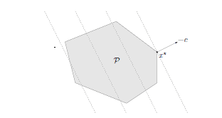
The geometric interpretation of an LP is illustrated in figure 4.4. The feasible set of the LP $(4.27)$ is a polyhedron $\mathcal{P}$; the problem is to minimize the affine function $c^{T} x+d$ (or, equivalently, the linear function $c^{T} x$ ) over $\mathcal{P}$.
Standard and inequality form linear programs
Two special cases of the LP $(4.27)$ are so widely encountered that they have been given separate names. In a standard form $L P$ the only inequalities are componen-
roblems 147
Figure $4.4$ Geometric interpretation of an LP. The feasible set $\mathcal{P}$, which is a polyhedron, is shaded. The objective $c^{T} x$ is linear, so its level curves are hyperplanes orthogonal to $c$ (shown as dashed lines). The point $x^{*}$ is optimal; it is the point in $\mathcal{P}$ as far ss possible in the direction $-c .$
twise nonnegativity constraints $x \succeq 0$ :
$$
\begin{array}{ll}
\text { minimize } & c^{T} x \
\text { subject to } & A x=b \
& x \geq 0
\end{array}
$$
If the LP has no equality constraints, it is called an inequality form LP, usually written as
$$
\begin{array}{ll}
\text { minimize } & c^{T} x \
\text { subject to } & A x \preceq b
\end{array}
$$
Converting LPs to standard form
It is sometimes useful to transform a general LP $(4.27)$ to one in standard form (4.28) (for example in order to use an algorithm for standard form LPs). The first step is to introduce slack variables $s_{1}$ for the inequalities, which results in
$$
\begin{array}{ll}
\text { minimize } & c^{T} x+d \
\text { subject to } & G x+s=h \
& A x=b \
& s \succeq 0 .
\end{array}
$$
The second step is to express the variable $x$ as the difference of two nonnegative variables $x^{+}$and $x^{-}$, i.e., $x=x^{+}-x^{-}, x^{+}, x^{-} \succeq 0$. This yields the problem
$$
\begin{array}{ll}
\operatorname{minimize} & e^{T} x^{+}-c^{T} x^{-}+d \
\text { subject to } & G x^{+}-G x^{-}+8=h \
& A x^{+}-A x^{-}=b \
& x^{+} \succeq 0, \quad x^{-} \succeq 0, \quad s \succeq 0,
\end{array}
$$
4 Convex optimization problems
148
which is an LP in standard form, with variables $x^{+}, x^{-}$, and $s$. (For equivalence of this problem and the original one $(4.27)$, see exercise $4.10 .$ )
These techniques for manipulating problems (along with many others we will see in the examples and exercises) can be used to formulate many problems as linear programs. With some abuse of terminology, it is common to refer to a problem that can be formulated as an LP as an LP, even if it does not have the form (4.27).
examples.
Diet problem
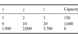
A healthy diet contains $m$ different nutrients in quantities at least equal to $b_{1}, \ldots$, $b_{m}$. We can compose such a diet by choosing nonnegative quantities $x_{1}, \ldots, x_{n}$ of $n$ different foods. One unit quantity of food $j$ contains an amount $a_{i j}$ of nutrient $i$, and has a cost of $c_{j}$. We want to determine the cheapest diet that satisfies the nutritional requirements. This problem can be formulated as the LP
$\begin{array}{ll}\text { minimize } & c^{T} x \ \text { subject to } & A x \succeq b \ & x \succeq 0\end{array}$
Several variations on this problem can also be formulated as LPs. For example, we can insist on an exact amount of a nutrient in the diet (which gives a linear equality constraint), or we can impose an upper bound on the amount of a nutrient, in addition to the lower bound as above.
Chebyshev center of a polyhedron
We consider the problem of finding the largest Euclidean ball that lies in a polyhedron described by linear inequalities,
$$
\mathcal{P}=\left{x \in \mathbf{R}^{n} \mid a_{i}^{T} x \leq b_{i}, i=1, \ldots, m\right} .
$$
(The center of the optimal ball is called the Chebyshev center of the polyhedron; it is the point deepest inside the polyhedron, ie., farthest from the boundary; see $\$ 8.5 .1 .$ ) We represent the ball as
$$
\mathcal{B}=\left{x_{c}+u \mid|u|_{2} \leq r\right} .
$$
The variables in the problem are the center $x_{c} \in \mathbf{R}^{n}$ and the radius $r$; we wish to maximize $r$ subject to the constraint $\mathcal{B} \subseteq \mathcal{P}$.
We start by considering the simpler constraint that $\mathcal{B}$ lies in one halfspace $a_{i}^{T} x \leq b_{i}$, i.e.,
$$
|u|_{2} \leq r \Longrightarrow a_{i}^{T}\left(x_{c}+u\right) \leq b_{i} .
$$
Since
$$
\sup \left{a_{i}^{T} u \mid|u|_{2} \leq r\right}=r\left|a_{i}\right|_{2}
$$
数值分析代考
当目标函数和约束函数都是仿射的时,这个问题被称为线性正数(LP)。一般线性规划具有以下形式
$$
\开始{数组}{ll}
\text { 最小化 } & c^{T} x+d \
\text { 服从 } & G x \preceq h \
& A x=b
\结束{数组}
twise 非负约束 $x \succeq 0$ :
$$
\开始{数组}{ll}
\text { 最小化 } & c^{T} x \
\text { 服从 } & A x=b \
& x \geq 0
\结束{数组}
$$
如果 LP 没有等式约束,则称为不等式形式 LP,通常写为
$$
\开始{数组}{ll}
\text { 最小化 } & c^{T} x \
\text { 服从 } & A x \preceq b
\结束{数组}
$$
将 LP 转换为标准格式
有时将一般 LP $(4.27)$ 转换为标准形式 (4.28) 是有用的(例如,为了使用标准形式 LP 的算法)。第一步是为不等式引入松弛变量 $s_{1}$,这导致
$$
\开始{数组}{ll}
\text { 最小化 } & c^{T} x+d \
\text { 服从 } & G x+s=h \
& A x=b \
& s \succeq 0 。
\结束{数组}
$$
第二步,将变量$x$表示为两个非负变量$x^{+}$和$x^{-}$的差,即$x=x^{+}-x^{-} , x^{+}, x^{-} \succeq 0$。这产生了问题
$$
\开始{数组}{ll}
\operatorname{最小化} & e^{T} x^{+}-c^{T} x^{-}+d \
\text { 服从 } & G x^{+}-G x^{-}+8=h \
& A x^{+}-A x^{-}=b \
& x^{+} \succeq 0, \quad x^{-} \succeq 0, \quad s \succeq 0,
\结束{数组}
$$
4 凸优化问题
148
这是标准形式的 LP,具有变量 $x^{+}、x^{-}$ 和 $s$。 (关于这个问题和原始问题 $(4.27)$ 的等价性,请参见练习 $4.10 .$ )
这些处理问题的技术(以及我们将在示例和练习中看到的许多其他技术)可用于将许多问题表述为线性程序。由于滥用了一些术语,通常将可以表述为 LP 的问题称为 LP,即使它不具有 (4.27) 形式。
$$
其中 $G \in \mathbf{R}^{m \times n}$ 和 $A \in \mathbf{R}^{p \times n}$。线性规划当然是凸优化问题。
在目标函数中省略常数 $d$ 是很常见的,因为它不会影响最优(或可行)集。由于我们可以最大化仿射目标 $c^{T} x+$ $d$,通过最小化 $-c^{T} xd$(仍然是凸的),我们还提到了具有仿射目标和约束函数的最大化问题作为一个LP。
LP 的几何解释如图 4.4 所示。 LP $(4.27)$ 的可行集是一个多面体 $\mathcal{P}$;问题是在 $\mathcal{P}$ 上最小化仿射函数 $c^{T} x+d$(或等价的线性函数 $c^{T} x$)。
标准和不等式形成线性规划
LP $(4.27)$ 的两个特殊情况非常普遍,以至于它们被赋予了不同的名称。在标准形式 $L P$ 中,唯一的不等式是分量
问题 147
图 $4.4$ LP 的几何解释。多面体的可行集 $\mathcal{P}$ 带有阴影。目标 $c^{T} x$ 是线性的,因此它的水平曲线是与 $c$ 正交的超平面(显示为虚线)。点 $x^{*}$ 是最优的;它是 $\mathcal{P}$ 中的点,尽可能在 $-c .$ 方向上
twise 非负约束 $x \succeq 0$ :
$$
\开始{数组}{ll}
\text { 最小化 } & c^{T} x \
\text { 服从 } & A x=b \
& x \geq 0
\结束{数组}
$$
如果 LP 没有等式约束,则称为不等式形式 LP,通常写为
$$
\开始{数组}{ll}
\text { 最小化 } & c^{T} x \
\text { 服从 } & A x \preceq b
\结束{数组}
$$
将 LP 转换为标准格式
有时将一般 LP $(4.27)$ 转换为标准形式 (4.28) 是有用的(例如,为了使用标准形式 LP 的算法)。第一步是为不等式引入松弛变量 $s_{1}$,这导致
$$
\开始{数组}{ll}
\text { 最小化 } & c^{T} x+d \
\text { 服从 } & G x+s=h \
& A x=b \
& s \succeq 0 。
\结束{数组}
$$
第二步,将变量$x$表示为两个非负变量$x^{+}$和$x^{-}$的差,即$x=x^{+}-x^{-} , x^{+}, x^{-} \succeq 0$。这产生了问题
$$
\开始{数组}{ll}
\operatorname{最小化} & e^{T} x^{+}-c^{T} x^{-}+d \
\text { 服从 } & G x^{+}-G x^{-}+8=h \
& A x^{+}-A x^{-}=b \
& x^{+} \succeq 0, \quad x^{-} \succeq 0, \quad s \succeq 0,
\结束{数组}
$$
4 凸优化问题
148
这是标准形式的 LP,具有变量 $x^{+}、x^{-}$ 和 $s$。 (关于这个问题和原始问题 $(4.27)$ 的等价性,请参见练习 $4.10 .$ )
这些处理问题的技术(以及我们将在示例和练习中看到的许多其他技术)可用于将许多问题表述为线性程序。由于滥用了一些术语,通常将可以表述为 LP 的问题称为 LP,即使它不具有 (4.27) 形式。
例子。
饮食问题
健康的饮食包含 $m$ 不同的 nu

数学代写| Chebyshev polynomials 数值分析代考 请认准UprivateTA™. UprivateTA™为您的留学生涯保驾护航。
时间序列分析代写
统计作业代写
随机过程代写
随机过程,是依赖于参数的一组随机变量的全体,参数通常是时间。 随机变量是随机现象的数量表现,其取值随着偶然因素的影响而改变。 例如,某商店在从时间t0到时间tK这段时间内接待顾客的人数,就是依赖于时间t的一组随机变量,即随机过程