物理代写| Orbits in Schwarzschild Spacetime 相对论代考
物理代写
6.4 Orbits in Schwarzschild Spacetime
6.4.1 The First Integrals
A test particle-a particle of small mass such that its gravitational field can be safely ignored in the given physical scenario-under no external forces (except gravitation-recall that in GR, gravity is not looked upon as a force) moves along a geodesic of the spacetime. If the particle has non-zero rest-mass then it moves along a timelike geodesic-the tangent to the geodesic at any point $u^{i}=d x^{i} / d s$ is a timelike vector, and we have $u^{i} u_{i}>0-$ in fact if $s$ is the arclength or $c$ times the proper time then $u^{i} u_{i}=1$. If the test particle has zero rest-mass like a photon, then the tangent to the geodesic is null, that is, if we define the tangent as $u^{i}=d x^{i} / d \lambda$ We take the parameter $\lambda$ to be an affine parameter which has been explained in Chapter $4 .$
Normally, to compute the geodesics, we need to solve the geodesic equations:
$$
\frac{\mathrm{d}^{2} x^{i}}{\mathrm{~d} \lambda^{2}}+\Gamma^{i}{ }_{j k} \frac{\mathrm{d} x^{j}}{\mathrm{~d} \lambda} \frac{\mathrm{d} x^{k}}{\mathrm{~d} \lambda}=0,
$$
where we have generically used $\lambda$. We may set $\lambda=s$ for the timelike geodesics. We need to solve these equations with boundary conditions or initial conditions.
However, for the Schwarzschild spacetime a first principle approach is more useful, because it has several symmetries-it is static, the metric is time independentand also it is spherically symmetric. Therefore, it makes sense to start from the variational principle and integrate the geodesic equations step by step, by first obtaining the first integrals and identifying the integration constants with physical quantities. We proceed as follows.
First of all, from spherical symmetry, the orbit (geodesic) must be confined to a plane. Because if the particle starts of from a given point and in a given direction, the particle must remain in the plane determined by the, initial space-time point, the tangent vector and $r=0$-otherwise one hemisphere would be chosen over the other, violating symmetry. We will orient the Schwarzschild coordinates in such a and obtain its extremum; hence we write:
$$
\delta \int\left(e^{v} c^{2} \dot{t}^{2}-e^{-v} \dot{r}^{2}-r^{2} \dot{\phi}^{2}\right) d s=0
$$
where the ‘dot’ denotes differentiation with respect to $s$. Thus $\dot{t}=d t / d s$ and so on. We have also considered timelike geodesics first because they are easier to understand. Note that the $\dot{\theta}=0$, because $\theta$ is set to be a constant, namely, $\pi / 2$, a consequence of spherical symmetry. Note that this can be rigorously proved from the geodesic equation for $\theta$. If we set $\theta=\pi / 2$ and $\dot{\theta}=0$ in the geodesic equation for $\theta$,
108
6 Schwarzschild Solution and Black Holes
we find that $\ddot{\theta}=0$, establishing that the particle does not leave the $\theta=\pi / 2$ plane. See Exercise $3 .$
We now use the Euler-Lagrange equations to obtain the orbits. Consider a function $F\left(\dot{x}^{i}, x^{k}\right)$ and we require:
$$
\delta \int F\left(\dot{x}^{i}, x^{k}\right) d s=0
$$
where the dot represents $d / d s$. This condition on the integral is converted into a differential condition by the Euler-Lagrange equations:
$$
\frac{d}{d s}\left(\frac{\partial F}{\partial \dot{x}^{i}}\right)-\frac{\partial F}{\partial x^{i}}=0
$$
Here we have $F=e^{v} c^{2} \dot{t}^{2}-e^{-v} \dot{r}^{2}-r^{2} \dot{\phi}^{2}$ and $x^{0}=c t$. If $F$ does not depend on explicitly on $x^{i}$ for some specific $i$, then,
$$
\frac{d}{d s}\left(\frac{\partial F}{\partial \dot{x}^{i}}\right)=0 \Rightarrow \frac{\partial F}{\partial \dot{x}^{i}}=\text { const. } \equiv p_{i}
$$
物理代考
=
6.4 史瓦西时空中的轨道
6.4.1 第一积分
一个测试粒子——一个小质量的粒子,使得它的引力场在给定的物理场景中可以安全地忽略——在没有外力的情况下(除了引力——回想一下,在 GR 中,引力不被视为一种力)沿着测地线移动的时空。如果粒子具有非零静止质量,则它沿着类时测地线移动——在任意点 $u^{i}=dx^{i} / ds$ 的测地线的切线是类时向量,我们有 $ u^{i} u_{i}>0-$ 实际上如果 $s$ 是弧长或 $c$ 乘以适当的时间,那么 $u^{i} u_{i}=1$。如果测试粒子像光子一样具有零静止质量,则测地线的切线为零,也就是说,如果我们将切线定义为 $u^{i}=dx^{i} / d \lambda$ 我们取参数 $\lambda$ 为仿射参数,已在第 $4 章中解释过。$
通常,要计算测地线,我们需要求解测地线方程:
$$
\frac{\mathrm{d}^{2} x^{i}}{\mathrm{~d} \lambda^{2}}+\Gamma^{i}{ }_{jk} \frac{\mathrm {d} x^{j}}{\mathrm{~d} \lambda} \frac{\mathrm{d} x^{k}}{\mathrm{~d} \lambda}=0,
$$
我们通常使用 $\lambda$。我们可以为类时测地线设置$\lambda=s$。我们需要用边界条件或初始条件来求解这些方程。
然而,对于 Schwarzschild 时空,第一原理方法更有用,因为它有几个对称性——它是静态的,度量是时间无关的,而且它是球对称的。因此,有必要从变分原理开始,逐步对测地线方程进行积分,首先获得第一个积分,然后用物理量确定积分常数。我们进行如下。
首先,从球对称性来看,轨道(测地线)必须限制在一个平面内。因为如果粒子从给定点和给定方向开始,则粒子必须保持在由初始时空点、切向量和 $r=0$ 确定的平面内,否则将选择一个半球而不是另一个,违反对称性。我们将Schwarzschild坐标定位在这样的a中并获得它的极值;因此我们写:
$$
\delta \int\left(e^{v} c^{2} \dot{t}^{2}-e^{-v} \dot{r}^{2}-r^{2} \dot {\phi}^{2}\right) ds=0
$$
其中“点”表示相对于 $s$ 的微分。因此 $\dot{t}=d t / d s$ 等等。我们还首先考虑了类时测地线,因为它们更容易理解。注意$\dot{\theta}=0$,因为$\theta$被设置为一个常数,即$\pi / 2$,这是球对称的结果。请注意,这可以从 $\theta$ 的测地线方程严格证明。如果我们在 $\theta$ 的测地线方程中设置 $\theta=\pi / 2$ 和 $\dot{\theta}=0$,
108
6 史瓦西解和黑洞
我们发现$\ddot{\theta}=0$,确定粒子没有离开$\theta=\pi / 2$ 平面。见练习 $3 .$
我们现在使用欧拉-拉格朗日方程来获得轨道。考虑一个函数 $F\left(\dot{x}^{i}, x^{k}\right)$,我们要求:
$$
\delta \int F\left(\dot{x}^{i}, x^{k}\right) d s=0
$$
其中点代表$d / d s$。积分条件通过欧拉-拉格朗日方程转换为微分条件:
$$
\frac{d}{ds}\left(\frac{\partial F}{\partial \dot{x}^{i}}\right)-\frac{\partial F}{\partial x^{i} }=0
$$
这里我们有 $F=e^{v} c^{2} \dot{t}^{2}-e^{-v} \dot{r}^{2}-r^{2} \dot{ \phi}^{2}$ 和 $x^{0}=ct$。如果对于某些特定的 $i$,$F$ 不明确依赖于 $x^{i}$,那么,
$$
\frac{d}{ds}\left(\frac{\partial F}{\partial \dot{x}^{i}}\right)=0 \Rightarrow \frac{\partial F}{\partial \dot {x}^{i}}=\text { 常量。 } \equiv p_{i}
$$

物理代考Gravity and Curvature of Space-Time 代写 请认准UprivateTA™. UprivateTA™为您的留学生涯保驾护航。
电磁学代考
物理代考服务:
物理Physics考试代考、留学生物理online exam代考、电磁学代考、热力学代考、相对论代考、电动力学代考、电磁学代考、分析力学代考、澳洲物理代考、北美物理考试代考、美国留学生物理final exam代考、加拿大物理midterm代考、澳洲物理online exam代考、英国物理online quiz代考等。
光学代考
光学(Optics),是物理学的分支,主要是研究光的现象、性质与应用,包括光与物质之间的相互作用、光学仪器的制作。光学通常研究红外线、紫外线及可见光的物理行为。因为光是电磁波,其它形式的电磁辐射,例如X射线、微波、电磁辐射及无线电波等等也具有类似光的特性。
大多数常见的光学现象都可以用经典电动力学理论来说明。但是,通常这全套理论很难实际应用,必需先假定简单模型。几何光学的模型最为容易使用。
相对论代考
上至高压线,下至发电机,只要用到电的地方就有相对论效应存在!相对论是关于时空和引力的理论,主要由爱因斯坦创立,相对论的提出给物理学带来了革命性的变化,被誉为现代物理性最伟大的基础理论。
流体力学代考
流体力学是力学的一个分支。 主要研究在各种力的作用下流体本身的状态,以及流体和固体壁面、流体和流体之间、流体与其他运动形态之间的相互作用的力学分支。
随机过程代写
随机过程,是依赖于参数的一组随机变量的全体,参数通常是时间。 随机变量是随机现象的数量表现,其取值随着偶然因素的影响而改变。 例如,某商店在从时间t0到时间tK这段时间内接待顾客的人数,就是依赖于时间t的一组随机变量,即随机过程