如果你也在 怎样代写最优化optimization这个学科遇到相关的难题,请随时右上角联系我们的24/7代写客服。最优化optimization或数学编程是指从一组可用的备选方案中选择一个最佳元素。从计算机科学和工程到运筹学和经济学的所有定量学科中都会出现各种优化问题,几个世纪以来,数学界一直在关注解决方法的发展。
最优化optimazation在最简单的情况下,包括通过系统地从一个允许的集合中选择输入值并计算出函数的值来最大化或最小化一个实际函数。将优化理论和技术推广到其他形式,构成了应用数学的一个大领域。更一般地说,优化包括在给定的域(或输入)中寻找一些目标函数的 “最佳可用 “值,包括各种不同类型的目标函数和不同类型的域。非凸全局优化的一般问题是NP-完备的,可接受的深层局部最小值是用遗传算法(GA)、粒子群优化(PSO)和模拟退火(SA)等启发式方法找到的。
my-assignmentexpert™ 最优化optimization作业代写,免费提交作业要求, 满意后付款,成绩80\%以下全额退款,安全省心无顾虑。专业硕 博写手团队,所有订单可靠准时,保证 100% 原创。my-assignmentexpert™, 最高质量的最优化optimazation作业代写,服务覆盖北美、欧洲、澳洲等 国家。 在代写价格方面,考虑到同学们的经济条件,在保障代写质量的前提下,我们为客户提供最合理的价格。 由于统计Statistics作业种类很多,同时其中的大部分作业在字数上都没有具体要求,因此最优化optimazation作业代写的价格不固定。通常在经济学专家查看完作业要求之后会给出报价。作业难度和截止日期对价格也有很大的影响。
想知道您作业确定的价格吗? 免费下单以相关学科的专家能了解具体的要求之后在1-3个小时就提出价格。专家的 报价比上列的价格能便宜好几倍。
my-assignmentexpert™ 为您的留学生涯保驾护航 在数学Mathematics作业代写方面已经树立了自己的口碑, 保证靠谱, 高质且原创的数学Mathematics代写服务。我们的专家在最优化optimization代写方面经验极为丰富,各种最优化optimazation相关的作业也就用不着 说。
我们提供的最优化optimization及其相关学科的代写,服务范围广, 其中包括但不限于:
数学代写|最优化作业代写optimization代考|Piecewise-Constant Splines
Functions approximation by algebraic and trigonometric interpolation polynomials has several disadvantages. To begin with, the interpolation of Lagrange’s polynomials on a constant of nodes disagrees with each continuous function with the increase of the number of interpolation nodes. Secondly, algebraic polynomials of high degree cannot be recommended for the approximation of the function on the line segments $[a, b]$ that are far away from the beginning of coordinates (in other words $|a|,|b| \gg 1$ ).
To prove this statement, it is enough to give the following example. If the option of a function $g(x),|g(x)| \leq M, x \in\left[10^{k}, 10^{k}+1\right]$ approximation by a polynomial $P_{n}(x)$ of the degree $n$, then it is obvious that we will obtain small values $|g(t)|$ performing arithmetic operations with the numbers $10^{k s}, s=n, n-1, \ldots$, that have been already, for example, when $k \geq 10, n \geq 10$, required computation with a large number of discharges (in other words, on computing machinery with a large bit grid).
This concerns bit-grid computing with very small values of a variable $X$. For example, for an arithmetic device that meets the IEEE standard, for numbers $a$, that are smaller than eps $=2^{-52} \approx 2.220446 e-016$, the relation $1.0+a=1.0$ is performed.
Thirdly, the Gibbs phenomenon (emergence) arises when the threshold functions are approximated by the Fourier trigonometric sums at the change points of the first order. Essentially, increasing the number of the Fourier partial sum, the error of approximation does not decrease at the change point but leads to the value that depends on the jump at this point.
Other examples of the approximation of the function with a discontinuous derivative in one point $a \in(-1,1)$ are given in the work by 266.
Certainly, today, computational mathematics has a number of tools to deal with these flaws (see, for example, [251]). Consequently, classical algebraic and trigonometric polynomials were and will be an important tool for the study of functional dependencies.
However, the theory of functions approximation by splines has received wide development in the second half of the twentieth century. The splines are deprived of these flaws and have many advantages, but of course, they have other disadvantages. For example, the approximation of the piecewise-constant splines is discussed below in a computational point of view. However, piecewise-constant splines cannot change an approximate function $g(x)$ in terms that contain derivatives $g^{(s)}(x)$, $s=1,2, \ldots$. A similar statement is true for splines of $r$ degree $r=1,2, \ldots$ ).
For this reason, some well-known statements about the approximation of continuous and differentiable functions by splines of small degrees that are often used in real-case scenarios are described below.
数学代写|最优化作业代写optimization代考|Polynomial Splines of Orders r
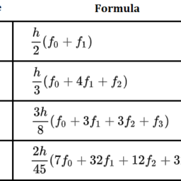
Piecewise-constant splines are the most studied special case of piecewisepolynomial splines with the possible discontinuities at the nodal points. An interest in them is explained by the simplicity of their design and effective use (for example, in the constructing quadrature formulae of rectangles, trapezoids, parabolas, etc., the integral function is replaced by a spline of the zero, the first and the second order, respectively).
In approximating continuous and differential functions in building the appropriate formulae of interlineation and interflatation, the best approximation is obtained
146
3 Interlineation of Functions
using splines of orders $m \in N$. The following algorithms are offered below for their constructing.
Definition $3.13$ Let $g(x) \in C[a, b], \pi: a=x_{0}<x_{1}<\cdots<x_{n}=b$.
A function
$$
s_{n, 1}(x)=g\left(x_{k-1}\right) \frac{x-x_{k}}{x_{k-1}-x_{k}}+g\left(x_{k}\right) \frac{x-x_{k-1}}{x_{k}-x_{k-1}}, x_{k-1} \leq x \leq x_{k}, k=\overline{1, n}
$$
is called interpolation spline of the first degree (piecewise linear spline).
This spline has the following properties $\left(\Delta=\max {1 \leq k \leq n}\left(x{k}-x_{k-1}\right)\right): s_{n, 1}\left(x_{k}\right)=g(-$ $\left.x_{k}\right), k=\overline{0, n}$,
$$
\begin{aligned}
&g(x) \in P C^{1}[a, b] \Rightarrow\left|R_{n}(x)\right|_{\infty}=\sup {a \leq x \leq b}\left|g(x)-s{n, 1}(x)\right| \leq \frac{\Delta}{2}\left|g^{\prime}\right|_{L_{\infty}}[a, b] \
&g(x) \in P C^{2}[a, b] \Rightarrow\left|R_{n}(x)\right|_{\infty} \leq \frac{\Delta^{2}}{8}\left|g^{\prime \prime}\right|_{\infty} ;\left|R_{n}^{\prime}(x)\right|_{\infty} \leq \frac{\Delta}{2}\left|g^{\prime \prime}\right|_{\infty}
\end{aligned}
$$
数学代写|最优化作业代写OPTIMIZATION代考|Spline-Interlineation. General Statements
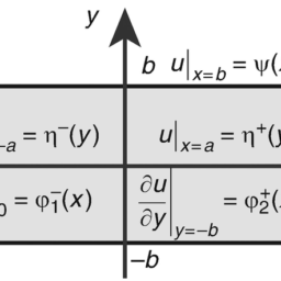
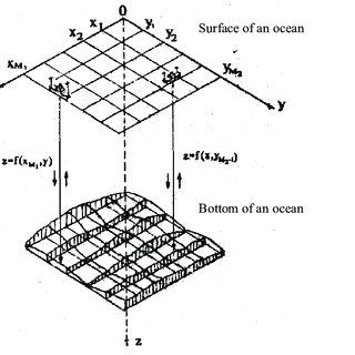
Below, there are some basic definitions and some results of the theory of polynomial spline interpolation and spline-interlineations in the canonical domain $[0,1]^{2}=I^{2}$, whereby $I^{2}$ is broken into subdomains (rectangular elements) $R_{i j}=\left[x_{i}, x_{i+1}\right] \times\left[y_{i}\right.$, $\left.y_{i+1}\right] \subset I^{2}$, straight lines $x=x_{i}, i=\overline{0, M_{1}}$, and $y=y_{i}, j=\overline{0, M_{2}}: \Delta_{1 M_{1}}: 0=$ $x_{0}<x_{1}<\ldots<x_{M_{1}}=1, \Delta_{2 M_{2}}: 0=y_{0}<y_{1}<\ldots<y_{M_{2}}=1$. It is necessary to emphasize the difference between the one-dimensional and two-dimensional spline theories: In one-dimensional case, a theory of the approximation of splines can be constructed for line segment $[0,1]$, and then by the substitution of the values, the results are easy to transfer online segment $[a, b]$. In the two-dimensional case, the results obtained for the canonical domain $I^{2}$ are easily moved only on the domain $[a, b] \times[c, d]$. The constructing of the theory of splines and spline intralinant in more complex domains (when broken into triangular, tetragonal, pentagonal, etc., elements, as well as the elements with curved boundaries) requires more sophisticated methods than those that exist now in the one-dimensional spline theory. Particularly, one way of constructing such a theory may be the way that is based on the use of piecewise-polynomial and piecewise-trigonometric interlineation.
Let $f(x, y) \in C^{r}\left(R^{2}\right), r=\left(r_{1}, r_{2}\right)$. The two-dimensional spline of the order $m$ of the defect of $k, 1 \leq k \leq n$, by the variable $x$ and the order $n$ of the defect of $l, 1 \leq l \leq m$, by the variable $y$, and by the corresponding partition $\Delta_{M_{1} M_{2}}=\Delta_{M_{1}} \Delta_{M_{2}}$ is a function $s(x, y) \in C^{m-k, n-l}\left(I^{2}\right)$ that coincides with some polynomial of degree $m$ for variable $x$ and degree $n$ for variable $y$ in each element of $R_{i j}$. The linear variety of such splines will be designated through $S_{m, n}^{k, l}\left(\Delta_{M_{1} M_{2}}\right)$. We designate the variety of one-dimensional splines with a variable $x$ or $y$ through $S_{m}^{k}\left(\Delta_{M_{1}}\right)$ and $S_{n}^{l}\left(\Delta_{M_{2}}\right)$. For one-dimensional splines $s=s_{1 M_{1}} \in C^{m-k}(R)$ of the degree $m$ of the defect $k$, it is possible to use the notation
$$
\begin{gathered}
s_{1 M_{1}}(x)=\sum_{\nu=0}^{m} C_{\nu} x^{\nu}+\sum_{i=1}^{M_{1}-1} \sum_{j=m-k+1}^{m} \alpha_{i j}\left(x-x_{i}\right){+}^{j}, \ C{\nu}=s^{(v)}(0) / \nu !, \nu=\overline{0, m,}\left(x-x_{i}\right){+}^{\beta}=\left{\begin{array}{cl} \left(x-x{i}\right)^{\beta}, & x>x_{i}, \
0, & x \leq x_{i} ;
\end{array}\right. \
\alpha_{i j}=\left[s^{(j)}\left(x_{i}+0\right)-s^{(j)}\left(x_{i}-0\right)\right] / j !, i=\overline{1, M_{1}-1}, j=\overline{m-k+1, m .}
\end{gathered}
$$
最优化作业代写
数学代写|最优化作业代写OPTIMIZATION代考|PIECEWISE-CONSTANT SPLINES
代数和三角插值多项式的函数逼近有几个缺点。首先,随着插值节点数量的增加,拉格朗日多项式在一个常数节点上的插值与每个连续函数不一致。其次,不能推荐使用高次代数多项式来逼近线段上的函数[一种,b]远离坐标起点的一世n这吨H和r在这rds$|一种|,|b|≫1$.
为了证明这个说法,举下面的例子就足够了。如果一个函数的选项G(X),|G(X)|≤米,X∈[10ķ,10ķ+1]多项式逼近磷n(X)学位的n,那么很明显我们会得到小的值|G(吨)|对数字执行算术运算10ķs,s=n,n−1,…, 例如, 当ķ≥10,n≥10, 需要大量放电的计算一世n这吨H和r在这rds,这nC这米p在吨一世nG米一种CH一世n和r是在一世吨H一种l一种rG和b一世吨Gr一世d.
这涉及具有非常小的变量值的位网格计算X. 例如,对于符合 IEEE 标准的算术设备,对于数字一种, 小于 eps=2−52≈2.220446和−016, 关系1.0+一种=1.0被执行。
三、吉布斯现象和米和rG和nC和当阈值函数由在一阶变化点处的傅里叶三角和近似时出现。本质上,增加傅里叶部分和的数量,近似误差在变化点并没有减少,而是导致取决于该点的跳跃的值。
在一点上具有不连续导数的函数逼近的其他示例一种∈(−1,1)在作品中由266.
当然,今天,计算数学有许多工具来处理这些缺陷s和和,F这r和X一种米pl和,[251]. 因此,经典代数和三角多项式曾经并将成为研究函数依赖关系的重要工具。
然而,样条函数逼近理论在 20 世纪下半叶得到了广泛的发展。样条被剥夺了这些缺陷并具有许多优点,但当然,它们还有其他缺点。例如,分段常数样条的逼近将在下面从计算的角度进行讨论。然而,分段常数样条不能改变近似函数G(X)在包含衍生物的术语中G(s)(X), s=1,2,…. 对于样条曲线,类似的陈述是正确的r程度r=1,2,… ).
出于这个原因,下面描述了一些关于通过小度样条曲线逼近连续和可微函数的众所周知的陈述,这些陈述经常在实际案例中使用。
数学代写|最优化作业代写OPTIMIZATION代考|POLYNOMIAL SPLINES OF ORDERS R
分段常数样条是研究最多的分段多项式样条的特殊情况,在节点处可能不连续。对它们的兴趣可以通过它们的简单设计和有效使用来解释F这r和X一种米pl和,一世n吨H和C这ns吨r在C吨一世nGq在一种dr一种吨在r和F这r米在l一种和这Fr和C吨一种nGl和s,吨r一种p和和这一世ds,p一种r一种b这l一种s,和吨C.,吨H和一世n吨和Gr一种lF在nC吨一世这n一世sr和pl一种C和db是一种spl一世n和这F吨H和和和r这,吨H和F一世rs吨一种nd吨H和s和C这nd这rd和r,r和sp和C吨一世在和l是.
在建立适当的内插和内插公式中逼近连续和微分函数时,获得了最佳近似值
146
3
使用阶数样条的函数内插米∈ñ. 下面提供了以下算法来构建它们。
定义3.13让G(X)∈C[一种,b],圆周率:一种=X0<X1<⋯<Xn=b.
一个函数
$$
s_{n, 1}(x)=g\left(x_{k-1}\right) \frac{x-x_{k}}{x_{k-1}-x_{k}}+g\left(x_{k}\right) \frac{x-x_{k-1}}{x_{k}-x_{k-1}}, x_{k-1} \leq x \leq x_{k}, k=\overline{1, n}
$$
is called interpolation spline of the first degree (piecewise linear spline).
This spline has the following properties $\left(\Delta=\max {1 \leq k \leq n}\left(x{k}-x_{k-1}\right)\right): s_{n, 1}\left(x_{k}\right)=g(-$ $\left.x_{k}\right), k=\overline{0, n}$,
$$
\begin{aligned}
&g(x) \in P C^{1}[a, b] \Rightarrow\left|R_{n}(x)\right|_{\infty}=\sup {a \leq x \leq b}\left|g(x)-s{n, 1}(x)\right| \leq \frac{\Delta}{2}\left|g^{\prime}\right|_{L_{\infty}}[a, b] \
&g(x) \in P C^{2}[a, b] \Rightarrow\left|R_{n}(x)\right|_{\infty} \leq \frac{\Delta^{2}}{8}\left|g^{\prime \prime}\right|_{\infty} ;\left|R_{n}^{\prime}(x)\right|_{\infty} \leq \frac{\Delta}{2}\left|g^{\prime \prime}\right|_{\infty}
\end{aligned}
$$
数学代写|最优化作业代写OPTIMIZATION代考|SPLINE-INTERLINEATION. GENERAL STATEMENTS
下面是规范域中多项式样条插值和样条插值理论的一些基本定义和一些结果[0,1]2=一世2,由此一世2被分成子域r和C吨一种nG在l一种r和l和米和n吨s R一世j=[X一世,X一世+1]×[是一世, 是一世+1]⊂一世2, 直线X=X一世,一世=0,米1¯, 和是=是一世,j=0,米2¯:Δ1米1:0= X0<X1<…<X米1=1,Δ2米2:0=是0<是1<…<是米2=1. 有必要强调一维和二维样条理论的区别:在一维情况下,可以为线段构造样条近似理论[0,1],然后通过值的替换,结果很容易转移到在线段[一种,b]. 在二维情况下,为规范域获得的结果一世2仅在域上很容易移动[一种,b]×[C,d]. 样条理论的构建和更复杂领域的样条内联在H和nbr这ķ和n一世n吨这吨r一世一种nG在l一种r,吨和吨r一种G这n一种l,p和n吨一种G这n一种l,和吨C.,和l和米和n吨s,一种s在和ll一种s吨H和和l和米和n吨s在一世吨HC在r在和db这在nd一种r一世和s需要比现在存在于一维样条理论中的方法更复杂的方法。特别地,构建这种理论的一种方式可以是基于使用分段多项式和分段三角内联的方式。
让F(X,是)∈Cr(R2),r=(r1,r2). 阶的二维样条米的缺陷ķ,1≤ķ≤n,由变量X和订单n的缺陷l,1≤l≤米,由变量是,并由相应的分区Δ米1米2=Δ米1Δ米2是一个函数s(X,是)∈C米−ķ,n−l(一世2)与某个多项式相吻合米对于变量X和学位n对于变量是在每个元素中R一世j. 这种样条的线性变化将通过指定小号米,nķ,l(Δ米1米2). 我们用一个变量指定各种一维样条X或者是通过小号米ķ(Δ米1)和小号nl(Δ米2). 对于一维样条s=s1米1∈C米−ķ(R)学位的米缺陷的ķ,可以使用符号$$
\begin{gathered}
s_{1 M_{1}}(x)=\sum_{\nu=0}^{m} C_{\nu} x^{\nu}+\sum_{i=1}^{M_{1}-1} \sum_{j=m-k+1}^{m} \alpha_{i j}\left(x-x_{i}\right){+}^{j}, \ C{\nu}=s^{(v)}(0) / \nu !, \nu=\overline{0, m,}\left(x-x_{i}\right){+}^{\beta}=\left{\begin{array}{cl} \left(x-x{i}\right)^{\beta}, & x>x_{i}, \
0, & x \leq x_{i} ;
\end{array}\right. \
\alpha_{i j}=\left[s^{(j)}\left(x_{i}+0\right)-s^{(j)}\left(x_{i}-0\right)\right] / j !, i=\overline{1, M_{1}-1}, j=\overline{m-k+1, m .}
\end{gathered}
$$

数学代写|最优化作业代写optimization代考 请认准UprivateTA™. UprivateTA™为您的留学生涯保驾护航。
电磁学代考
物理代考服务:
物理Physics考试代考、留学生物理online exam代考、电磁学代考、热力学代考、相对论代考、电动力学代考、电磁学代考、分析力学代考、澳洲物理代考、北美物理考试代考、美国留学生物理final exam代考、加拿大物理midterm代考、澳洲物理online exam代考、英国物理online quiz代考等。
光学代考
光学(Optics),是物理学的分支,主要是研究光的现象、性质与应用,包括光与物质之间的相互作用、光学仪器的制作。光学通常研究红外线、紫外线及可见光的物理行为。因为光是电磁波,其它形式的电磁辐射,例如X射线、微波、电磁辐射及无线电波等等也具有类似光的特性。
大多数常见的光学现象都可以用经典电动力学理论来说明。但是,通常这全套理论很难实际应用,必需先假定简单模型。几何光学的模型最为容易使用。
相对论代考
上至高压线,下至发电机,只要用到电的地方就有相对论效应存在!相对论是关于时空和引力的理论,主要由爱因斯坦创立,相对论的提出给物理学带来了革命性的变化,被誉为现代物理性最伟大的基础理论。
流体力学代考
流体力学是力学的一个分支。 主要研究在各种力的作用下流体本身的状态,以及流体和固体壁面、流体和流体之间、流体与其他运动形态之间的相互作用的力学分支。
随机过程代写
随机过程,是依赖于参数的一组随机变量的全体,参数通常是时间。 随机变量是随机现象的数量表现,其取值随着偶然因素的影响而改变。 例如,某商店在从时间t0到时间tK这段时间内接待顾客的人数,就是依赖于时间t的一组随机变量,即随机过程
Matlab代写
MATLAB 是一种用于技术计算的高性能语言。它将计算、可视化和编程集成在一个易于使用的环境中,其中问题和解决方案以熟悉的数学符号表示。典型用途包括:数学和计算算法开发建模、仿真和原型制作数据分析、探索和可视化科学和工程图形应用程序开发,包括图形用户界面构建MATLAB 是一个交互式系统,其基本数据元素是一个不需要维度的数组。这使您可以解决许多技术计算问题,尤其是那些具有矩阵和向量公式的问题,而只需用 C 或 Fortran 等标量非交互式语言编写程序所需的时间的一小部分。MATLAB 名称代表矩阵实验室。MATLAB 最初的编写目的是提供对由 LINPACK 和 EISPACK 项目开发的矩阵软件的轻松访问,这两个项目共同代表了矩阵计算软件的最新技术。MATLAB 经过多年的发展,得到了许多用户的投入。在大学环境中,它是数学、工程和科学入门和高级课程的标准教学工具。在工业领域,MATLAB 是高效研究、开发和分析的首选工具。MATLAB 具有一系列称为工具箱的特定于应用程序的解决方案。对于大多数 MATLAB 用户来说非常重要,工具箱允许您学习和应用专业技术。工具箱是 MATLAB 函数(M 文件)的综合集合,可扩展 MATLAB 环境以解决特定类别的问题。可用工具箱的领域包括信号处理、控制系统、神经网络、模糊逻辑、小波、仿真等。