如果你也在 怎样代写计算金融Computational finance这个学科遇到相关的难题,请随时右上角联系我们的24/7代写客服。计算金融Computational finance是应用计算机科学的一个分支,处理金融中的实际利益问题。一些略有不同的定义是研究目前用于金融的数据和算法以及实现金融模型或系统的计算机程序的数学。
计算金融Computational finance强调实用的数字方法,而不是数学证明,并侧重于直接应用于经济分析的技术。它是数学金融学和数字方法之间的一个跨学科领域。两个主要领域是金融证券公允价值的有效和准确计算以及随机时间序列的建模。计算金融作为一门学科的诞生可以追溯到20世纪50年代初的哈里-马科维茨。马科维茨将投资组合的选择问题设想为均值-方差优化的一个练习。这需要比当时更多的计算机能力,所以他致力于研究有用的近似解决方案的算法。
my-assignmentexpert™ 计算金融Computational finance作业代写,免费提交作业要求, 满意后付款,成绩80\%以下全额退款,安全省心无顾虑。专业硕 博写手团队,所有订单可靠准时,保证 100% 原创。my-assignmentexpert™, 最高质量的计算金融Computational finance作业代写,服务覆盖北美、欧洲、澳洲等 国家。 在代写价格方面,考虑到同学们的经济条件,在保障代写质量的前提下,我们为客户提供最合理的价格。 由于统计Statistics作业种类很多,同时其中的大部分作业在字数上都没有具体要求,因此计算金融Computational finance作业代写的价格不固定。通常在经济学专家查看完作业要求之后会给出报价。作业难度和截止日期对价格也有很大的影响。
想知道您作业确定的价格吗? 免费下单以相关学科的专家能了解具体的要求之后在1-3个小时就提出价格。专家的 报价比上列的价格能便宜好几倍。
my-assignmentexpert™ 为您的留学生涯保驾护航 在计算金融project作业代写方面已经树立了自己的口碑, 保证靠谱, 高质且原创的计算金融project代写服务。我们的专家在计算金融Computational finance代写方面经验极为丰富,各种计算金融Computational finance相关的作业也就用不着 说。
我们提供的计算金融Computational finance及其相关学科的代写,服务范围广, 其中包括但不限于:
金融代写|计算金融project代写Computational finance代考|Boundary Conditions
Let the spatial domain $\left(S_{\min }, S_{\max }\right)$ be bounded. For ease of presentation it will always be assumed that the general convection-diffusionreaction equation (2.1) is provided with a Dirichlet condition at the lower boundary $s=S_{\min }$,
$$
u\left(S_{\min }, t\right)=a_{0}(t) \quad(0 \leq t \leq T),
$$
where $a_{0}$ is a given function.
Let $m \geq 3$ be any given integer and let a spatial mesh width and spatial grid points be given by
$$
h=\frac{S_{\max }-S_{\min }}{m} \quad \text { and } \quad s_{i}=S_{\min }+i h \quad(i=0,1,2, \ldots, m) .
$$
金融代写|计算金融PROJECT代写COMPUTATIONAL FINANCE代考|Nonuniform Grids
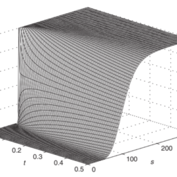
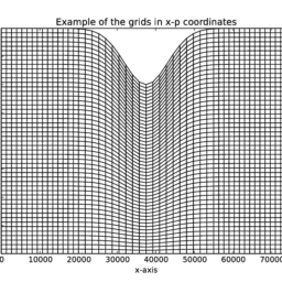
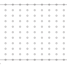
As alluded to in Chapter 4 , it is often natural and beneficial to use nonuniform spatial grids in financial applications. For the numerical experiments we consider the smooth, nonuniform grid constructed in Example 4.2.1. As an illustration Figure $5.4$ shows the corresponding spatial grid points for $m=50$. It is clear that the grid is densest around the strike. This forms the region of interest in practice, as asset prices do not lie far away in general from the chosen strike.
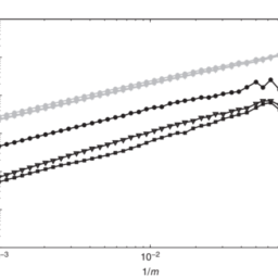
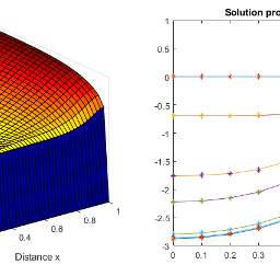
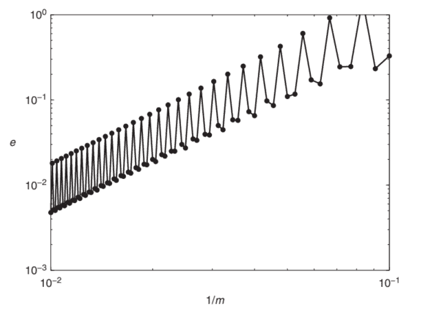
For the semidiscretization the second-order central formulas from Chapter 4 for nonuniform grids are employed and cell averaging is applied as in the previous section. Recall that for nonuniform grids there are two finite difference formulas, $\mathrm{A}$ and $\mathrm{B}$, for the convection part, see (4.6) and (4.7). Figure $5.5$ displays the spatial errors $e(m)$ versus $1 / m$, where bullets correspond to formula A and squares to formula B. As a first main observation, with both formulas secondorder convergence of the spatial discretization is attained. Next, the approximations obtained by using formula $B$ are slightly more accurate than those obtained by using formula A. Comparing to Figure $5.3$, the approximations on the nonuniform grid are with both formulas substantially more accurate than those on the uniform grid. In particular, with formula B the gain in accuracy in the present example is more than a factor of $4 .$
金融代写|计算金融PROJECT代写COMPUTATIONAL FINANCE代考|Boundary Conditions
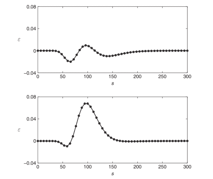
In this section we take a closer look at the influence of the boundary condition at $s=S_{\max }$. Boundary conditions that are imposed in practice at the truncated boundaries usually introduce an error, as they are not satisfied by the exact option value function. Thus the spatial error component $\varepsilon_{m}(\mathrm{~m})$ is nonzero in general.
In the situation of Sections $5.1$ and $5.2$, where a Dirichlet condition has been applied, a direct computation using the Black-Scholes formula (1.6) yields that $\varepsilon_{m}(m)$ is equal to $1.8 \times 10^{-5}$ for all $m$. This error is always dominated in the experiments in these sections by the
errors around the strike and, consequently, it does not show up in Figures $5.2,5.3,5.5$. The same is found when the Dirichlet condition (2.5) at $s=S_{\max }$ is replaced by the Neumann condition (2.6) or the linear condition (2.7) and the pertinent Figures $5.2,5.3,5.5$ remain visually unchanged.
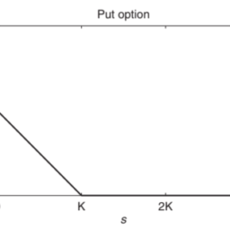
In the experiments so far, $10 \leq m \leq 100$. If the number of grid points is further increased, then $\varepsilon_{m}(m)$ eventually starts to dominate the spatial error over the domain $\left[0, S_{\max }\right]$ and the norm of the spatial error, $e(m)$, levels off at $\left|\varepsilon_{m}(m)\right|$. In practice, however, only a region of interest, such as $\frac{1}{2} K<s<\frac{3}{2} K$, is of importance; compare Section 2.3. A natural alternative measure for spatial accuracy is therefore the (norm of the) spatial discretization error on a region of interest,
$$
e^{R O I}(m)=\max \left{\left|\varepsilon_{i}(m)\right|: 0 \leq i \leq m, \frac{1}{2} K<s_{i}<\frac{3}{2} K\right} .
$$
计算金融代写
金融代写|计算金融PROJECT代写COMPUTATIONAL FINANCE代考|BOUNDARY CONDITIONS
让空间域(小号分钟,小号最大限度)有界。为了便于演示,总是假设一般的对流-扩散反应方程2.1在下边界处具有狄利克雷条$$
u\left(S_{\min }, t\right)=a_{0}(t) \quad(0 \leq t \leq T),
$$
where $a_{0}$ is a given function.
Let $m \geq 3$ be any given integer and let a spatial mesh width and spatial grid points be given by
$$
h=\frac{S_{\max }-S_{\min }}{m} \quad \text { and } \quad s_{i}=S_{\min }+i h \quad(i=0,1,2, \ldots, m) .
$$
金融代写|计算金融PROJECT代写COMPUTATIONAL FINANCE代考|NONUNIFORM GRIDS
正如第 4 章所提到的,在金融应用中使用非均匀空间网格通常是自然而有益的。对于数值实验,我们考虑示例 4.2.1 中构建的平滑、非均匀网格。如图所示5.4显示相应的空间网格点米=50. 很明显,罢工周围的网格最密集。这在实践中形成了感兴趣的区域,因为资产价格通常不会远离所选的罢工。
对于半离散化,使用了来自第 4 章的非均匀网格的二阶中心公式,并且像上一节一样应用了单元平均。回想一下,对于非均匀网格,有两个有限差分公式,一种和乙,对流部分,见4.6和4.7. 数字5.5显示空间误差和(米)相对1/米,其中子弹对应于公式 A,正方形对应于公式 B。作为第一个主要观察结果,两个公式都实现了空间离散化的二阶收敛。接下来,使用公式得到的近似值乙比使用公式 A 得到的结果稍微准确一些。5.3,非均匀网格上的近似值在两个公式中都比均匀网格上的近似值要准确得多。特别是,对于公式 B,本示例中的准确度增益超过了4.
金融代写|计算金融PROJECT代写COMPUTATIONAL FINANCE代考|BOUNDARY CONDITIONS
在本节中,我们将仔细研究边界条件的影响s=小号最大限度. 实际上在截断边界处施加的边界条件通常会引入错误,因为它们不满足确切的期权价值函数。因此空间误差分量e米( 米)一般不为零。
在分段的情况下5.1和5.2,其中应用了 Dirichlet 条件,使用 Black-Scholes 公式的直接计算1.6产生e米(米)等于1.8×10⁻⁵对全部米. 在这些部分的实验中,这个错误总是由
罢工周围的错误主导,因此,它没有出现在图中5.2,5.3,5.5. 当 Dirichlet 条件2.5在s=小号最大限度被诺依曼条件取代2.6或线性条件2.7和相关的数字5.2,5.3,5.5视觉上保持不变。
在迄今为止的实验中,10≤米≤100. 如果进一步增加网格点数,则e米(米)最终开始主导域上的空间误差[0,小号最大限度]和空间误差的范数,和(米), 稳定在|e米(米)|. 然而,在实践中,只有一个感兴趣的区域,例如12ķ<s<32ķ, 很重要;比较第 2.3 节。因此,空间精度的一个自然替代度量是n这r米这F吨H和感兴趣区域的空间离散化误差,
e^{R O I}(m)=\max \left{\left|\varepsilon_{i}(m)\right|: 0 \leq i \leq m, \frac{1}{2} K<s_{i }<\frac{3}{2} K\right} 。

金融代写|计算金融project代写Computational finance代考 请认准UprivateTA™. UprivateTA™为您的留学生涯保驾护航。
电磁学代考
物理代考服务:
物理Physics考试代考、留学生物理online exam代考、电磁学代考、热力学代考、相对论代考、电动力学代考、电磁学代考、分析力学代考、澳洲物理代考、北美物理考试代考、美国留学生物理final exam代考、加拿大物理midterm代考、澳洲物理online exam代考、英国物理online quiz代考等。
光学代考
光学(Optics),是物理学的分支,主要是研究光的现象、性质与应用,包括光与物质之间的相互作用、光学仪器的制作。光学通常研究红外线、紫外线及可见光的物理行为。因为光是电磁波,其它形式的电磁辐射,例如X射线、微波、电磁辐射及无线电波等等也具有类似光的特性。
大多数常见的光学现象都可以用经典电动力学理论来说明。但是,通常这全套理论很难实际应用,必需先假定简单模型。几何光学的模型最为容易使用。
相对论代考
上至高压线,下至发电机,只要用到电的地方就有相对论效应存在!相对论是关于时空和引力的理论,主要由爱因斯坦创立,相对论的提出给物理学带来了革命性的变化,被誉为现代物理性最伟大的基础理论。
流体力学代考
流体力学是力学的一个分支。 主要研究在各种力的作用下流体本身的状态,以及流体和固体壁面、流体和流体之间、流体与其他运动形态之间的相互作用的力学分支。
随机过程代写
随机过程,是依赖于参数的一组随机变量的全体,参数通常是时间。 随机变量是随机现象的数量表现,其取值随着偶然因素的影响而改变。 例如,某商店在从时间t0到时间tK这段时间内接待顾客的人数,就是依赖于时间t的一组随机变量,即随机过程
Matlab代写
MATLAB 是一种用于技术计算的高性能语言。它将计算、可视化和编程集成在一个易于使用的环境中,其中问题和解决方案以熟悉的数学符号表示。典型用途包括:数学和计算算法开发建模、仿真和原型制作数据分析、探索和可视化科学和工程图形应用程序开发,包括图形用户界面构建MATLAB 是一个交互式系统,其基本数据元素是一个不需要维度的数组。这使您可以解决许多技术计算问题,尤其是那些具有矩阵和向量公式的问题,而只需用 C 或 Fortran 等标量非交互式语言编写程序所需的时间的一小部分。MATLAB 名称代表矩阵实验室。MATLAB 最初的编写目的是提供对由 LINPACK 和 EISPACK 项目开发的矩阵软件的轻松访问,这两个项目共同代表了矩阵计算软件的最新技术。MATLAB 经过多年的发展,得到了许多用户的投入。在大学环境中,它是数学、工程和科学入门和高级课程的标准教学工具。在工业领域,MATLAB 是高效研究、开发和分析的首选工具。MATLAB 具有一系列称为工具箱的特定于应用程序的解决方案。对于大多数 MATLAB 用户来说非常重要,工具箱允许您学习和应用专业技术。工具箱是 MATLAB 函数(M 文件)的综合集合,可扩展 MATLAB 环境以解决特定类别的问题。可用工具箱的领域包括信号处理、控制系统、神经网络、模糊逻辑、小波、仿真等。