如果你也在 怎样代写计算金融Computational finance这个学科遇到相关的难题,请随时右上角联系我们的24/7代写客服。计算金融Computational finance是应用计算机科学的一个分支,处理金融中的实际利益问题。一些略有不同的定义是研究目前用于金融的数据和算法以及实现金融模型或系统的计算机程序的数学。
计算金融Computational finance强调实用的数字方法,而不是数学证明,并侧重于直接应用于经济分析的技术。它是数学金融学和数字方法之间的一个跨学科领域。两个主要领域是金融证券公允价值的有效和准确计算以及随机时间序列的建模。计算金融作为一门学科的诞生可以追溯到20世纪50年代初的哈里-马科维茨。马科维茨将投资组合的选择问题设想为均值-方差优化的一个练习。这需要比当时更多的计算机能力,所以他致力于研究有用的近似解决方案的算法。
my-assignmentexpert™ 计算金融Computational finance作业代写,免费提交作业要求, 满意后付款,成绩80\%以下全额退款,安全省心无顾虑。专业硕 博写手团队,所有订单可靠准时,保证 100% 原创。my-assignmentexpert™, 最高质量的计算金融Computational finance作业代写,服务覆盖北美、欧洲、澳洲等 国家。 在代写价格方面,考虑到同学们的经济条件,在保障代写质量的前提下,我们为客户提供最合理的价格。 由于统计Statistics作业种类很多,同时其中的大部分作业在字数上都没有具体要求,因此计算金融Computational finance作业代写的价格不固定。通常在经济学专家查看完作业要求之后会给出报价。作业难度和截止日期对价格也有很大的影响。
想知道您作业确定的价格吗? 免费下单以相关学科的专家能了解具体的要求之后在1-3个小时就提出价格。专家的 报价比上列的价格能便宜好几倍。
my-assignmentexpert™ 为您的留学生涯保驾护航 在计算金融project作业代写方面已经树立了自己的口碑, 保证靠谱, 高质且原创的计算金融project代写服务。我们的专家在计算金融Computational finance代写方面经验极为丰富,各种计算金融Computational finance相关的作业也就用不着 说。
我们提供的计算金融Computational finance及其相关学科的代写,服务范围广, 其中包括但不限于:
金融代写|计算金融project代写Computational finance代考|Explicit Method
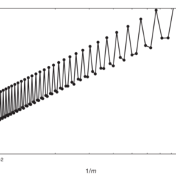
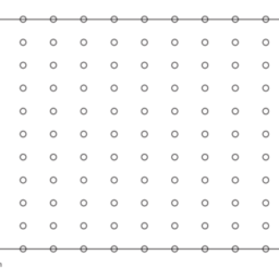
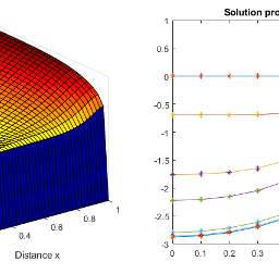
First consider application of the forward Euler method. Set $m=50$ for the spatial grid and choose $N=75$ and $N=80$ time steps. Figure 8.1 displays the two obtained fully discrete approximations at $t=T$. The top graph shows the result for $N=75$. Clearly, this numerical solution is very poor, with excessively large positive and large negative values. The bottom graph shows the result for $N=80$. This forms a visually fine numerical solution; compare Figure $1.2$ for the graph of the exact solution. Selecting smaller numbers of time steps than $N=75$ leads to similar incorrect results as in the top of Figure $8.1$, whereas taking larger numbers than $N=80$ yields decent results. Hence, there appears to be a critical, minimal number of steps that is required, equal to about $N=80$. Considering next $m=100,200,400$ numerical experiments reveal critical numbers of time steps approximately equal to $N=330,1330,5350$, respectively. These numbers grow fast and appear to be directly proportional to $\mathrm{m}^{2}$.
To gain insight into the above observation we take a look at the eigenvalue condition (7.9), with $m$ replaced by $v$. Computation in Matlab of the eigenvalues $\lambda_{1}, \lambda_{2}, \ldots, \lambda_{v}$ of the pertinent $v \times v$ matrix $A$ indicates that, for each value $m$ considered, they all lie on the negative real axis and, with the corresponding value $N$ found above and $\Delta t=T / N$,
it holds that
$$
\min {1 \leq k \leq \nu} \Delta t \lambda{k} \in[-2.02,-1.99]
$$
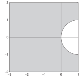
The intersection of the stability region $\mathcal{S}$ of the forward Euler method with the negative real axis is the interval $[-2,0]$. Hence, for each $m$, the corresponding value $N$ above is very close to the minimal value $N$ for which the eigenvalue condition (7.9) is fulfilled. If the number of time steps is smaller than this critical value, then an unstable behaviour of the forward Euler method is to be expected, which is indeed what the numerical experiments indicate. In particular, if $m=50$ and $N=75$, then $\min {k} \Delta t \lambda{k}=-2.15$. This point clearly lies outside of $\mathcal{S}$, explaining the poor fully discrete approximation in this case.
Subsequent numerical experiments suggest that there is a stable behaviour of the forward Euler method whenever the number of time steps is larger than the critical value. Even though the present matrix $A$ is nonnormal, fulfilment of (7.9) thus appears to guarantee conditional stability. As alluded to before, the relevant step size restriction is of the form $\Delta t=\mathcal{O}\left(\mathrm{m}^{-2}\right)$. This is of the same kind as obtained in Chapter 7 in the case of the pure model diffusion equation with periodic condition. For practical applications, where efficiency is crucial, this step size restriction is too severe.
金融代写|计算金融PROJECT代写COMPUTATIONAL FINANCE代考|Implicit Methods
In view of the unfavourable experience with the forward Euler method, we consider in this section numerical experiments with two implicit methods, backward Euler and Crank-Nicolson. It turns out that with these two methods always a visually fine numerical solution is obtained, for any given number of time steps. This forms a striking, positive difference with the case of the forward Euler method. Relatedly, since the backward Euler and Crank-Nicolson methods are both $A$-stable, condition (7.9) is now always fulfilled whenever the eigenvalues of the matrix $A$ lie in the left-half of the complex plane.
To study the convergence behaviour of the two implicit methods, we consider the temporal discretization error at $t=T=N \Delta t$ defined by
$\widehat{\varepsilon}(\Delta t ; m)=\left(\widehat{\varepsilon}{i}(\Delta t ; m)\right){i=0}^{m} \quad$ with $\quad \widehat{\varepsilon}{i}(\Delta t ; m)=U{i}(T)-U_{N, i} \quad(0 \leq i \leq m)$, and maximum norm
$$
\widehat{e}(\Delta t ; m)=\max \left{\left|\widehat{\varepsilon}_{i}(\Delta t ; m)\right|: 0 \leq i \leq m\right} .
$$
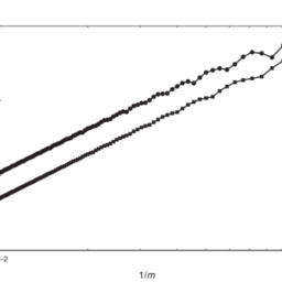
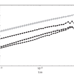
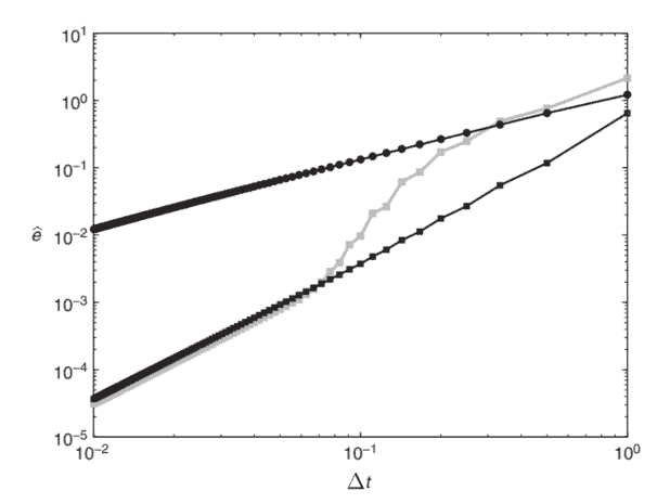
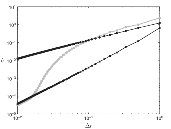
Figures $8.2$ and $8.3$ display for $m=50$ and $m=200$, respectively, the values $\widehat{e}(\Delta t ; m)$ versus $\Delta t$ in double logarithmic scale for all $1 \leq N \leq 100$. The results for backward Euler are shown by dark bullets and those for Crank-Nicolson by light squares. The dark squares are discussed below.
For the backward Euler method one observes that the (norm of the) temporal discretization errors are all bounded from above by a moderate constant and decrease monotonically as $N$ increases. The slope of the line through the results for backward Euler is $1.0$, which indicates that $\widehat{e}(\Delta t ; m)$ is approximately equal to $\widehat{C} \Delta t$ with constant $\widehat{C}$ independent of $N$. This corresponds to a first-order convergence behaviour, as expected. Comparing next the lines for $m=50$ and $m=200$ in Figures $8.2$ and $8.3$ for backward Euler, no vertical shift is observable, indicating that $\widehat{C}$ is independent of $m$, as desired; see Section 7.2. Additional numerical experiments with larger values $m$ support this main conclusion.
计算金融代写
金融代写|计算金融PROJECT代写COMPUTATIONAL FINANCE代考|EXPLICIT METHOD
首先考虑前向欧拉方法的应用。放米=50对于空间网格并选择ñ=75和ñ=80时间步长。图 8.1 显示了两个获得的完全离散近似值吨=吨. 上图显示了结果ñ=75. 显然,这个数值解很差,正值过大,负值过大。底部图表显示了结果ñ=80. 这形成了视觉上精细的数值解;比较图1.2对于精确解的图。选择的时间步数少于ñ=75导致与图顶部类似的错误结果8.1,而取大于ñ=80产生不错的结果。因此,似乎需要一个关键的、最少的步骤,大约等于ñ=80. 接下来考虑米=100,200,400数值实验揭示了时间步长的临界数量大约等于ñ=330,1330,5350, 分别。这些数字增长迅速,似乎与米2.
为了深入了解上述观察,我们看一下特征值条件7.9, 和米取而代之在. Matlab中特征值的计算λ1,λ2,…,λ在相关的在×在矩阵一种表示,对于每个值米考虑到,它们都位于负实轴上,并且具有相应的值ñ发现上面和Δ吨=吨/ñ,
它认为
$$
\min {1 \leq k \leq \nu} \Delta t \lambda {k} \in−2.02,−1.99
$$
稳定区域的交点小号负实轴的正向欧拉法的区间是[−2,0]. 因此,对于每个米, 对应的值ñ以上非常接近最小值ñ特征值条件7.9被履行。如果时间步数小于该临界值,则可以预期前向欧拉方法的不稳定行为,这确实是数值实验所表明的。特别是,如果米=50和ñ=75, 那么 $\min {k} \Delta t \lambda {k}=-2.15.吨H一世sp这一世n吨Cl和一种rl是l一世和s这在吨s一世d和这F\mathcal{S}$,解释了这种情况下糟糕的完全离散近似。
随后的数值实验表明,只要时间步数大于临界值,前向 Euler 方法的行为就会稳定。即使现在的矩阵一种是非正态的,满足7.9因此似乎保证了条件稳定性。如前所述,相关步长限制的形式为Δ吨=这(米−2). 这与第 7 章在具有周期条件的纯模型扩散方程的情况下获得的相同。对于效率至关重要的实际应用,此步长限制过于严格。
金融代写|计算金融PROJECT代写COMPUTATIONAL FINANCE代考|IMPLICIT METHODS
鉴于前向 Euler 方法的不利经验,我们在本节中考虑使用两种隐式方法的数值实验,即后向 Euler 和 Crank-Nicolson。事实证明,对于任何给定数量的时间步,使用这两种方法总是可以获得视觉上精细的数值解。这与前向欧拉方法的情况形成了显着的积极差异。相关地,由于后向 Euler 和 Crank-Nicolson 方法都是一种-稳定,状态7.9现在总是满足矩阵的特征值一种位于复平面的左半边。
为了研究两种隐式方法的收敛行为,我们考虑时间离散化误差吨=吨=ñΔ吨由
$A$-stable, condition (7.9) is now always fulfilled whenever the eigenvalues of the matrix $A$ lie in the left-half of the complex plane.
To study the convergence behaviour of the two implicit methods, we consider the temporal discretization error at $t=T=N \Delta t$ defined by
$\widehat{\varepsilon}(\Delta t ; m)=\left(\widehat{\varepsilon}{i}(\Delta t ; m)\right){i=0}^{m} \quad$ with $\quad \widehat{\varepsilon}{i}(\Delta t ; m)=U{i}(T)-U_{N, i} \quad(0 \leq i \leq m)$, and maximum norm
$$
\widehat{e}(\Delta t ; m)=\max \left{\left|\widehat{\varepsilon}_{i}(\Delta t ; m)\right|: 0 \leq i \leq m\right} .
$$
Figures $8.2$ and $8.3$ display for $m=50$ and $m=200$, respectively, the values $\widehat{e}(\Delta t ; m)$ versus $\Delta t$ in double logarithmic scale for all $1 \leq N \leq 100$.。后向 Euler 的结果用黑色子弹表示,Crank-Nicolson 的结果用浅色方块表示。下面讨论黑色方块。
对于后向欧拉方法,我们观察到n这r米这F吨H和时间离散化误差都由一个适度的常数从上面限定,并且随着ñ增加。通过反向欧拉结果的直线斜率为1.0,这表明和^(Δ吨;米)大约等于C^Δ吨与常数C^独立于ñ. 正如预期的那样,这对应于一阶收敛行为。比较下一行米=50和米=200在图中8.2和8.3对于后向欧拉,没有观察到垂直偏移,表明C^独立于米, 如预期的; 见第 7.2 节。具有较大值的附加数值实验米支持这个主要结论。

金融代写|计算金融project代写Computational finance代考 请认准UprivateTA™. UprivateTA™为您的留学生涯保驾护航。
电磁学代考
物理代考服务:
物理Physics考试代考、留学生物理online exam代考、电磁学代考、热力学代考、相对论代考、电动力学代考、电磁学代考、分析力学代考、澳洲物理代考、北美物理考试代考、美国留学生物理final exam代考、加拿大物理midterm代考、澳洲物理online exam代考、英国物理online quiz代考等。
光学代考
光学(Optics),是物理学的分支,主要是研究光的现象、性质与应用,包括光与物质之间的相互作用、光学仪器的制作。光学通常研究红外线、紫外线及可见光的物理行为。因为光是电磁波,其它形式的电磁辐射,例如X射线、微波、电磁辐射及无线电波等等也具有类似光的特性。
大多数常见的光学现象都可以用经典电动力学理论来说明。但是,通常这全套理论很难实际应用,必需先假定简单模型。几何光学的模型最为容易使用。
相对论代考
上至高压线,下至发电机,只要用到电的地方就有相对论效应存在!相对论是关于时空和引力的理论,主要由爱因斯坦创立,相对论的提出给物理学带来了革命性的变化,被誉为现代物理性最伟大的基础理论。
流体力学代考
流体力学是力学的一个分支。 主要研究在各种力的作用下流体本身的状态,以及流体和固体壁面、流体和流体之间、流体与其他运动形态之间的相互作用的力学分支。
随机过程代写
随机过程,是依赖于参数的一组随机变量的全体,参数通常是时间。 随机变量是随机现象的数量表现,其取值随着偶然因素的影响而改变。 例如,某商店在从时间t0到时间tK这段时间内接待顾客的人数,就是依赖于时间t的一组随机变量,即随机过程
Matlab代写
MATLAB 是一种用于技术计算的高性能语言。它将计算、可视化和编程集成在一个易于使用的环境中,其中问题和解决方案以熟悉的数学符号表示。典型用途包括:数学和计算算法开发建模、仿真和原型制作数据分析、探索和可视化科学和工程图形应用程序开发,包括图形用户界面构建MATLAB 是一个交互式系统,其基本数据元素是一个不需要维度的数组。这使您可以解决许多技术计算问题,尤其是那些具有矩阵和向量公式的问题,而只需用 C 或 Fortran 等标量非交互式语言编写程序所需的时间的一小部分。MATLAB 名称代表矩阵实验室。MATLAB 最初的编写目的是提供对由 LINPACK 和 EISPACK 项目开发的矩阵软件的轻松访问,这两个项目共同代表了矩阵计算软件的最新技术。MATLAB 经过多年的发展,得到了许多用户的投入。在大学环境中,它是数学、工程和科学入门和高级课程的标准教学工具。在工业领域,MATLAB 是高效研究、开发和分析的首选工具。MATLAB 具有一系列称为工具箱的特定于应用程序的解决方案。对于大多数 MATLAB 用户来说非常重要,工具箱允许您学习和应用专业技术。工具箱是 MATLAB 函数(M 文件)的综合集合,可扩展 MATLAB 环境以解决特定类别的问题。可用工具箱的领域包括信号处理、控制系统、神经网络、模糊逻辑、小波、仿真等。