如果你也在 怎样代写微积分Calculus 这个学科遇到相关的难题,请随时右上角联系我们的24/7代写客服。微积分Calculus 最初被称为无穷小微积分或 “无穷小的微积分”,是对连续变化的数学研究,就像几何学是对形状的研究,而代数是对算术运算的概括研究一样。
微积分Calculus 它有两个主要分支,微分和积分;微分涉及瞬时变化率和曲线的斜率,而积分涉及数量的累积,以及曲线下或曲线之间的面积。这两个分支通过微积分的基本定理相互关联,它们利用了无限序列和无限数列收敛到一个明确定义的极限的基本概念 。17世纪末,牛顿(Isaac Newton)和莱布尼兹(Gottfried Wilhelm Leibniz)独立开发了无限小数微积分。后来的工作,包括对极限概念的编纂,将这些发展置于更坚实的概念基础上。今天,微积分在科学、工程和社会科学中得到了广泛的应用。
微积分Calculus 代写,免费提交作业要求, 满意后付款,成绩80\%以下全额退款,安全省心无顾虑。专业硕 博写手团队,所有订单可靠准时,保证 100% 原创。 最高质量的微积分Calculus 作业代写,服务覆盖北美、欧洲、澳洲等 国家。 在代写价格方面,考虑到同学们的经济条件,在保障代写质量的前提下,我们为客户提供最合理的价格。 由于作业种类很多,同时其中的大部分作业在字数上都没有具体要求,因此微积分Calculus 作业代写的价格不固定。通常在专家查看完作业要求之后会给出报价。作业难度和截止日期对价格也有很大的影响。
同学们在留学期间,都对各式各样的作业考试很是头疼,如果你无从下手,不如考虑my-assignmentexpert™!
my-assignmentexpert™提供最专业的一站式服务:Essay代写,Dissertation代写,Assignment代写,Paper代写,Proposal代写,Proposal代写,Literature Review代写,Online Course,Exam代考等等。my-assignmentexpert™专注为留学生提供Essay代写服务,拥有各个专业的博硕教师团队帮您代写,免费修改及辅导,保证成果完成的效率和质量。同时有多家检测平台帐号,包括Turnitin高级账户,检测论文不会留痕,写好后检测修改,放心可靠,经得起任何考验!
想知道您作业确定的价格吗? 免费下单以相关学科的专家能了解具体的要求之后在1-3个小时就提出价格。专家的 报价比上列的价格能便宜好几倍。
我们在数学Mathematics代写方面已经树立了自己的口碑, 保证靠谱, 高质且原创的数学Mathematics代写服务。我们的专家在微积分Calculus Assignment代写方面经验极为丰富,各种微积分Calculus Assignment相关的作业也就用不着 说。
数学代写|微积分代写Calculus代考|Area and Estimating with Finite Sums
The basis for formulating definite integrals is the construction of approximations by finite sums. In this section we consider three examples of this process: finding the area under a graph, the distance traveled by a moving object, and the average value of a function. Although we have yet to define precisely what we mean by the area of a general region in the plane, or the average value of a function over a closed interval, we do have intuitive ideas of what these notions mean. We begin our approach to integration by approximating these quantities with simpler finite sums related to these intuitive ideas. We then consider what happens when we take more and more terms in the summation process. In subsequent sections we look at taking the limit of these sums as the number of terms goes to infinity, which leads to a precise definition of the definite integral.
Area
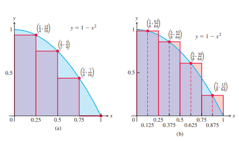
Suppose we want to find the area of the shaded region $R$ that lies above the $x$-axis, below the graph of $y=1-x^2$, and between the vertical lines $x=0$ and $x=1$ (see Figure 5.1).
Unfortunately, there is no simple geometric formula for calculating the areas of general shapes having curved boundaries like the region $R$. How, then, can we find the area of $R$ ?
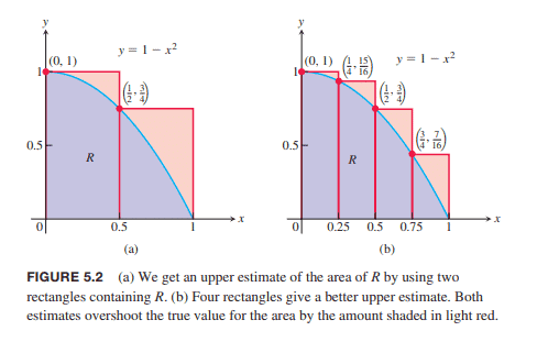
While we do not yet have a method for determining the exact area of $R$, we can approximate it in a simple way. Figure 5.2a shows two rectangles that together contain the region $R$. Each rectangle has width $1 / 2$ and they have heights 1 and $3 / 4$ (left to right). The height of each rectangle is the maximum value of the function $f$ in each subinterval. Because the function $f$ is decreasing, the height is its value at the left endpoint of the subinterval of $[0,1]$ that forms the base of the rectangle. The total area of the two rectangles approximates the area $A$ of the region $R$ :
$$
A \approx 1 \cdot \frac{1}{2}+\frac{3}{4} \cdot \frac{1}{2}=\frac{7}{8}=0.875
$$
This estimate is larger than the true area $A$ since the two rectangles contain $R$. We say that 0.875 is an upper sum because it is obtained by taking the height of the rectangle corresponding to the maximum (uppermost) value of $f(x)$ over points $x$ lying in the base of each rectangle. In Figure $5.2 \mathrm{~b}$, we improve our estimate by using four thinner rectangles, each of width $1 / 4$, which taken together contain the region $R$. These four rectangles give the approximation
$$
A \approx 1 \cdot \frac{1}{4}+\frac{15}{16} \cdot \frac{1}{4}+\frac{3}{4} \cdot \frac{1}{4}+\frac{7}{16} \cdot \frac{1}{4}=\frac{25}{32}=0.78125
$$
which is still greater than $A$ since the four rectangles contain $R$.
Suppose instead we use four rectangles contained inside the region $R$ to estimate the area, as in Figure 5.3a. Each rectangle has width $1 / 4$ as before, but the rectangles are shorter and lie entirely beneath the graph of $f$. The function $f(x)=1-x^2$ is decreasing on $[0,1]$, so the height of each of these rectangles is given by the value of $f$ at the right endpoint of the subinterval forming its base. The fourth rectangle has zero height and therefore contributes no area. Summing these rectangles, whose heights are the minimum value of $f(x)$ over points $x$ in the rectangle’s base, gives a lower sum approximation to the area:
$$
A \approx \frac{15}{16} \cdot \frac{1}{4}+\frac{3}{4} \cdot \frac{1}{4}+\frac{7}{16} \cdot \frac{1}{4}+0 \cdot \frac{1}{4}=\frac{17}{32}=0.53125 .
$$
数学代写|微积分代写Calculus代考|Distance Traveled
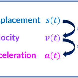
Suppose we know the velocity function $v(t)$ of a car that moves straight down a highway without changing direction, and we want to know how far it traveled between times $t=a$ and $t=b$. The position function $s(t)$ of the car has derivative $v(t)$. If we can find an antiderivative $F(t)$ of $v(t)$ then we can find the car’s position function $s(t)$ by setting $s(t)=F(t)+C$. The distance traveled can then be found by calculating the change in position, $s(b)-s(a)=F(b)-F(a)$. However, if the velocity is known only by the readings at various times of a speedometer on the car, then we have no formula from which to obtain an antiderivative for the velocity. So what do we do in this situation?
When we don’t know an antiderivative for the velocity $v(t)$, we can approximate the distance traveled by using finite sums in a way similar to the area estimates that we discussed before. We subdivide the interval $[a, b]$ into short time intervals and assume that the velocity on each subinterval is fairly constant. Then we approximate the distance traveled on each time subinterval with the usual distance formula
$$
\text { distance }=\text { velocity } \times \text { time }
$$
and add the results across $[a, b]$.
Suppose the subdivided interval looks like
with the subintervals all of equal length $\Delta t$. Pick a number $t_1$ in the first interval. If $\Delta t$ is so small that the velocity barely changes over a short time interval of duration $\Delta t$, then the distance traveled in the first time interval is about $v\left(t_1\right) \Delta t$. If $t_2$ is a number in the second interval, the distance traveled in the second time interval is about $v\left(t_2\right) \Delta t$. The sum of the distances traveled over all the time intervals is
$$
D \approx v\left(t_1\right) \Delta t+v\left(t_2\right) \Delta t+\cdots+v\left(t_n\right) \Delta t,
$$
where $n$ is the total number of subintervals. This sum is only an approximation to the true distance $D$, but the approximation increases in accuracy as we take more and more subintervals.
微积分代写
数学代写|微积分代写Calculus代考|Area and Estimating with Finite Sums
定积分公式的基础是用有限和构造近似。在本节中,我们将考虑这个过程的三个例子:寻找图下的面积,移动物体走过的距离,以及函数的平均值。虽然我们还没有精确地定义平面上一般区域的面积,或者函数在封闭区间上的平均值是什么意思,但我们对这些概念的含义有直观的认识。我们通过用与这些直观概念相关的更简单的有限和来近似这些量来开始我们的积分方法。然后我们考虑在求和过程中取越来越多的项会发生什么。在后面几节中,我们将讨论当项数趋于无穷时,求这些和的极限,从而得出定积分的精确定义。
面积
假设我们想要找到位于$x$ -轴上方、$y=1-x^2$图下方、垂直线条$x=0$和$x=1$之间的阴影区域$R$的面积(参见图5.1)。
不幸的是,没有简单的几何公式来计算具有弯曲边界的一般形状的面积,如$R$区域。那么,我们如何求出$R$的面积呢?
虽然我们还没有确定$R$的确切面积的方法,但我们可以用一种简单的方法来近似它。图5.2a显示了两个矩形,它们一起包含区域$R$。每个矩形的宽度为$1 / 2$,高度为1和$3 / 4$(从左到右)。每个矩形的高度是函数$f$在每个子区间中的最大值。因为函数$f$是递减的,所以高度是它在构成矩形底的$[0,1]$子区间的左端点处的值。两个矩形的总面积近似于区域$R$的面积$A$:
$$
A \approx 1 \cdot \frac{1}{2}+\frac{3}{4} \cdot \frac{1}{2}=\frac{7}{8}=0.875
$$
这个估计值比真实面积$A$大,因为两个矩形包含$R$。我们说0.875是一个上和,因为它是通过取每个矩形底部的点$x$上$f(x)$的最大值(最上端)对应的矩形的高度得到的。在图$5.2 \mathrm{~b}$中,我们通过使用四个更细的矩形来改进我们的估计,每个矩形的宽度为$1 / 4$,它们加在一起包含区域$R$。这四个矩形给出了近似
$$
A \approx 1 \cdot \frac{1}{4}+\frac{15}{16} \cdot \frac{1}{4}+\frac{3}{4} \cdot \frac{1}{4}+\frac{7}{16} \cdot \frac{1}{4}=\frac{25}{32}=0.78125
$$
它仍然大于$A$,因为这四个矩形包含$R$。
假设我们使用包含在区域$R$中的四个矩形来估计面积,如图5.3a所示。与之前一样,每个矩形的宽度为$1 / 4$,但矩形更短,并且完全位于$f$的图形下方。函数$f(x)=1-x^2$在$[0,1]$上递减,因此每个矩形的高度由构成其底的子区间右端点处的$f$的值给出。第四个矩形的高度为零,因此不占面积。将这些矩形加起来,其高度是矩形底部$f(x)$除以$x$点的最小值,得到面积的一个更小的和近似值:
$$
A \approx \frac{15}{16} \cdot \frac{1}{4}+\frac{3}{4} \cdot \frac{1}{4}+\frac{7}{16} \cdot \frac{1}{4}+0 \cdot \frac{1}{4}=\frac{17}{32}=0.53125 .
$$
数学代写|微积分代写Calculus代考|Distance Traveled
假设我们知道一辆车在高速公路上直行而不改变方向的速度函数$v(t)$,我们想知道它在时间$t=a$和$t=b$之间走了多远。小车的位置函数$s(t)$有一个导数$v(t)$。如果我们可以找到$v(t)$的不定积分$F(t)$,那么我们可以通过设置$s(t)=F(t)+C$找到汽车的位置函数$s(t)$。经过的距离可以通过计算位置的变化来计算,$s(b)-s(a)=F(b)-F(a)$。然而,如果速度只能通过汽车上的速度计在不同时间的读数来知道,那么我们就没有公式可以从中得到速度的不定积分。在这种情况下我们该怎么做?
当我们不知道速度$v(t)$的不定积分时,我们可以用有限和来近似移动的距离,类似于我们之前讨论过的面积估计。我们将区间$[a, b]$细分为较短的时间区间,并假设每个子区间上的速度相当恒定。然后我们用通常的距离公式来近似每个时间子区间上的距离
$$
\text { distance }=\text { velocity } \times \text { time }
$$
并将结果添加到$[a, b]$。
假设细分的区间是这样的
子区间的长度都相等$\Delta t$。在第一个间隔中选择一个数字$t_1$。如果$\Delta t$很小,速度在一个很短的时间间隔$\Delta t$内几乎没有变化,那么在第一个时间间隔内走过的距离大约是$v\left(t_1\right) \Delta t$。如果$t_2$是第二个时间间隔内的一个数字,则第二个时间间隔内走过的距离约为$v\left(t_2\right) \Delta t$。在所有时间间隔内移动的距离之和是
$$
D \approx v\left(t_1\right) \Delta t+v\left(t_2\right) \Delta t+\cdots+v\left(t_n\right) \Delta t,
$$
其中$n$为子区间的总数。这个和只是真实距离$D$的近似值,但是当我们取越来越多的子区间时,近似值的精度会增加。

数学代写|微积分代写Calculus代考 请认准UprivateTA™. UprivateTA™为您的留学生涯保驾护航。
微观经济学代写
微观经济学是主流经济学的一个分支,研究个人和企业在做出有关稀缺资源分配的决策时的行为以及这些个人和企业之间的相互作用。my-assignmentexpert™ 为您的留学生涯保驾护航 在数学Mathematics作业代写方面已经树立了自己的口碑, 保证靠谱, 高质且原创的数学Mathematics代写服务。我们的专家在图论代写Graph Theory代写方面经验极为丰富,各种图论代写Graph Theory相关的作业也就用不着 说。
线性代数代写
线性代数是数学的一个分支,涉及线性方程,如:线性图,如:以及它们在向量空间和通过矩阵的表示。线性代数是几乎所有数学领域的核心。
博弈论代写
现代博弈论始于约翰-冯-诺伊曼(John von Neumann)提出的两人零和博弈中的混合策略均衡的观点及其证明。冯-诺依曼的原始证明使用了关于连续映射到紧凑凸集的布劳威尔定点定理,这成为博弈论和数学经济学的标准方法。在他的论文之后,1944年,他与奥斯卡-莫根斯特恩(Oskar Morgenstern)共同撰写了《游戏和经济行为理论》一书,该书考虑了几个参与者的合作游戏。这本书的第二版提供了预期效用的公理理论,使数理统计学家和经济学家能够处理不确定性下的决策。
微积分代写
微积分,最初被称为无穷小微积分或 “无穷小的微积分”,是对连续变化的数学研究,就像几何学是对形状的研究,而代数是对算术运算的概括研究一样。
它有两个主要分支,微分和积分;微分涉及瞬时变化率和曲线的斜率,而积分涉及数量的累积,以及曲线下或曲线之间的面积。这两个分支通过微积分的基本定理相互联系,它们利用了无限序列和无限级数收敛到一个明确定义的极限的基本概念 。
计量经济学代写
什么是计量经济学?
计量经济学是统计学和数学模型的定量应用,使用数据来发展理论或测试经济学中的现有假设,并根据历史数据预测未来趋势。它对现实世界的数据进行统计试验,然后将结果与被测试的理论进行比较和对比。
根据你是对测试现有理论感兴趣,还是对利用现有数据在这些观察的基础上提出新的假设感兴趣,计量经济学可以细分为两大类:理论和应用。那些经常从事这种实践的人通常被称为计量经济学家。
Matlab代写
MATLAB 是一种用于技术计算的高性能语言。它将计算、可视化和编程集成在一个易于使用的环境中,其中问题和解决方案以熟悉的数学符号表示。典型用途包括:数学和计算算法开发建模、仿真和原型制作数据分析、探索和可视化科学和工程图形应用程序开发,包括图形用户界面构建MATLAB 是一个交互式系统,其基本数据元素是一个不需要维度的数组。这使您可以解决许多技术计算问题,尤其是那些具有矩阵和向量公式的问题,而只需用 C 或 Fortran 等标量非交互式语言编写程序所需的时间的一小部分。MATLAB 名称代表矩阵实验室。MATLAB 最初的编写目的是提供对由 LINPACK 和 EISPACK 项目开发的矩阵软件的轻松访问,这两个项目共同代表了矩阵计算软件的最新技术。MATLAB 经过多年的发展,得到了许多用户的投入。在大学环境中,它是数学、工程和科学入门和高级课程的标准教学工具。在工业领域,MATLAB 是高效研究、开发和分析的首选工具。MATLAB 具有一系列称为工具箱的特定于应用程序的解决方案。对于大多数 MATLAB 用户来说非常重要,工具箱允许您学习和应用专业技术。工具箱是 MATLAB 函数(M 文件)的综合集合,可扩展 MATLAB 环境以解决特定类别的问题。可用工具箱的领域包括信号处理、控制系统、神经网络、模糊逻辑、小波、仿真等。