如果你也在 怎样代写有限元方法finite differences method 这个学科遇到相关的难题,请随时右上角联系我们的24/7代写客服。有限元方法finite differences method在数值分析中,是一类通过用有限差分逼近导数解决微分方程的数值技术。空间域和时间间隔(如果适用)都被离散化,或被分成有限的步骤,通过解决包含有限差分和附近点的数值的代数方程来逼近这些离散点的解的数值。
有限元方法finite differences method有限差分法将可能是非线性的常微分方程(ODE)或偏微分方程(PDE)转换成可以用矩阵代数技术解决的线性方程系统。现代计算机可以有效地进行这些线性代数计算,再加上其相对容易实现,使得FDM在现代数值分析中得到了广泛的应用。今天,FDM与有限元方法一样,是数值解决PDE的最常用方法之一。
有限元方法finite differences method作业代写,免费提交作业要求, 满意后付款,成绩80\%以下全额退款,安全省心无顾虑。专业硕 博写手团队,所有订单可靠准时,保证 100% 原创。 最高质量的有限元方法finite differences method作业代写,服务覆盖北美、欧洲、澳洲等 国家。 在代写价格方面,考虑到同学们的经济条件,在保障代写质量的前提下,我们为客户提供最合理的价格。 由于统计Statistics作业种类很多,同时其中的大部分作业在字数上都没有具体要求,因此有限元方法finite differences method作业代写的价格不固定。通常在经济学专家查看完作业要求之后会给出报价。作业难度和截止日期对价格也有很大的影响。
同学们在留学期间,都对各式各样的作业考试很是头疼,如果你无从下手,不如考虑my-assignmentexpert™!
my-assignmentexpert™提供最专业的一站式服务:Essay代写,Dissertation代写,Assignment代写,Paper代写,Proposal代写,Proposal代写,Literature Review代写,Online Course,Exam代考等等。my-assignmentexpert™专注为留学生提供Essay代写服务,拥有各个专业的博硕教师团队帮您代写,免费修改及辅导,保证成果完成的效率和质量。同时有多家检测平台帐号,包括Turnitin高级账户,检测论文不会留痕,写好后检测修改,放心可靠,经得起任何考验!
想知道您作业确定的价格吗? 免费下单以相关学科的专家能了解具体的要求之后在1-3个小时就提出价格。专家的 报价比上列的价格能便宜好几倍。
我们在数学Mathematics代写方面已经树立了自己的口碑, 保证靠谱, 高质且原创的数学Mathematics代写服务。我们的专家在微积分Calculus Assignment代写方面经验极为丰富,各种微积分Calculus Assignment相关的作业也就用不着 说。
数学代写|有限元方法作业代写finite differences method代考|Finite Element Model of Bars and Cables
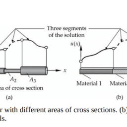
The average transverse deflection $u(x)$ of a cable (also termed rope or string) made of elastic material is also governed by an equation of the form:
$$
-\frac{d}{d x}\left(a \frac{d u}{d x}\right)=f(x)
$$
where $a$ is the uniform tension in the cable and $f$ is the distributed transverse force. Equation (4.4.1) is a special case of Eq. (3.4.1), with $c=0$. Therefore, the finite element equations presented in (3.4.32b) and (3.4.33) are valid (with $c=0$ ) for cables.
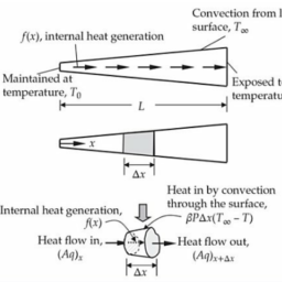
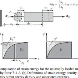
For axial deformation of bars, we also consider the effect of temperature increase (from a room temperature) on the strain, while presuming that the material properties are unaffected by the temperature change. The equations governing axial deformation of a bar are (see Example 1.2.3)
Equilibrium: $\quad-\frac{d(A \sigma)}{d x}=f(x)$
Kinematics: $\varepsilon=\frac{d u}{d x}-\alpha T$
Hooke’s law: $\sigma=E \varepsilon$
where $\sigma(x)$ denotes the axial stress $\left(\mathrm{N} / \mathrm{m}^2=\mathrm{Pa}\right), \varepsilon(x)(\mathrm{m} / \mathrm{m})$ is the axial strain, $u(x)$ is the axial displacement $(\mathrm{m}), T(x)$ is the temperature rise from a reference value $\left({ }^{\circ} \mathrm{C}\right), E=E(x)$ is the modulus of elasticity $(\mathrm{Pa}), \alpha(x)$ is the thermal coefficient of expansion $\left(1 /{ }^{\circ} \mathrm{C}\right), A=A(x)$ is the area of cross section of the bar $\left(\mathrm{m}^2\right)$, and $f(x)$ is the body force $(\mathrm{N} / \mathrm{m})$. It should be recalled that Eq. (4.4.2b) is derived under the assumption that the stress on any cross section is uniform.
When $\sigma$ and $\varepsilon$ are eliminated using Eqs. (4.4.2b) and (4.4.2c), Eq. (4.4.2a) can be expressed solely in terms of the displacement $u$ as
$$
-\frac{d}{d x}\left[E A\left(\frac{d u}{d x}-\alpha T\right)\right]=f(x)
$$
In deriving the weak form of Eq. (4.4.3), we must preserve the physical meaning of the secondary variable and integrate by parts the entire expression inside the square brackets:
$$
0=\int_{x_a^e}^{x_b^e}\left[E_c A_c \frac{d w}{d x}\left(\frac{d u^e}{d x}-\alpha_c T_c\right)-w f(x)\right] d x-Q_1^e w\left(x_a^e\right)-Q_2^e w\left(x_b^e\right)
$$
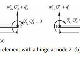
where $Q_1^e$ and $Q_2^e$ are the forces at the left and right ends of the element:
$$
Q_1^e=\left[-E_e A_e\left(\frac{d u_h^e}{d x}-\alpha_e T_e\right)\right]{x_e^e}, Q_2^e=\left[E_e A_e\left(\frac{d u_h^e}{d x}-\alpha_e T_e\right)\right]{x_b^e}
$$
The finite element model is
$$
\begin{gathered}
\mathbf{K}^e \mathbf{u}^e=\mathbf{f}^e+\mathbf{Q}^e \
K_{i j}^e=\int_{x_a^e}^{x_b^e} E_e A_e \frac{d \psi_i^e}{d x} \frac{d \psi_j^e}{d x} d x, \quad f_i^e=\int_{x_a^e}^{x_b^e}\left(f \psi_i^e+E_e A_e \alpha_e T_e \frac{d \psi_i^e}{d x}\right) d x
\end{gathered}
$$
Values of various integrals presented in Table 3.7.1 facilitate the computation of the element matrices in Eq. (4.4.5b).
数学代写|有限元方法作业代写finite differences method代考|Governing Equation
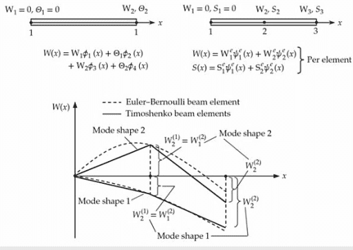
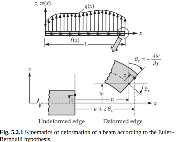
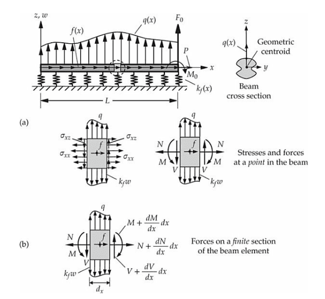
The Euler-Bernoulli beam theory (EBT) is based on the assumption that plane cross sections perpendicular to the axis of the beam remain plane, rigid, and perpendicular to the axis after deformation. Under the EBT hypothesis, the displacements of a point $(x, 0, z)$ in the beam along the three coordinate directions are
$$
u_x=u(x)+z \theta_x(x), u_y=0, u_z=w(x), \quad \theta_x \equiv-\frac{d w}{d x}
$$
where $\left(u_x, u_y, u_z\right)$ are the components of the displacement vector $\mathbf{u}$ referred to a rectangular Cartesian coordinate system, and $(u, w)$ are the axial and transverse displacements (measured in meters) of a point on the $x$-axis (i.e., at $z=0)$. Here $\theta x(x)=-(d w / d x)$ denotes the (clockwise) rotation about the $y$ axis of a straight line originally perpendicular to the $x$-axis, as shown in Fig. 5.2.1. Under the assumption of infinitesimal strains, the only nonzero strain $(\mathrm{m} / \mathrm{m})$ component is
$$
\varepsilon_{x x}=\frac{d u}{d x}-\alpha T+z \frac{d \theta_x}{d x}=\frac{d u}{d x}-\alpha T-z \frac{d^2 w}{d x^2}
$$
where $\alpha$ is the thermal coefficient of expansion and $T$ is the temperature rise, both of which are assumed to be functions of $x$ but not $z$. Using the uniaxial stress-strain relation, the axial stress $\left(\mathrm{N} / \mathrm{m}^2\right)$ in the beam is given by
$$
\sigma_{x x}=E\left(\frac{d u}{d x}-\alpha T+z \frac{d \theta_x}{d x}\right)=E\left(\frac{d u}{d x}-\alpha T-z \frac{d^2 w}{d x^2}\right)
$$
where $E=E(x)$ denotes the modulus of elasticity $\left(\mathrm{N} / \mathrm{m}^2\right)$. For a homogeneous beam, $E$ is a constant. We note that the shear stress $\sigma_{x z}$ computed from the constitutive equation is zero because the shear strain is zero: $\gamma_{x z}=\theta_x+$ $(d w / d x)=0$. However, in reality the shear stress and hence shear force cannot be zero because transverse loads induce transverse shear stresses. Therefore, the shear force is determined using the equilibrium equations.
有限元方法代写
数学代写|有限元方法作业代写finite differences method代考|Finite Element Model of Bars and Cables
平均横向挠度 $u(x)$ 由弹性材料制成的索(也称为绳或弦)的长度也由如下形式的方程决定:
$$
-\frac{d}{d x}\left(a \frac{d u}{d x}\right)=f(x)
$$
where $a$ 缆索上的张力是否一致 $f$ 为横向分布力。式(4.4.1)是式(3.4.1)的特例,其中 $c=0$. 因此,式(3.4.32b)和式(3.4.33)给出的有限元方程是有效的 $c=0$ )用于电缆。
对于棒的轴向变形,我们还考虑了温度升高(从室温开始)对应变的影响,同时假设材料性能不受温度变化的影响。控制杆轴向变形的方程为(见例1.2.3)
平衡: $\quad-\frac{d(A \sigma)}{d x}=f(x)$
运动学: $\varepsilon=\frac{d u}{d x}-\alpha T$
胡克定律: $\sigma=E \varepsilon$
where $\sigma(x)$ 为轴向应力 $\left(\mathrm{N} / \mathrm{m}^2=\mathrm{Pa}\right), \varepsilon(x)(\mathrm{m} / \mathrm{m})$ 为轴向应变, $u(x)$ 为轴向位移 $(\mathrm{m}), T(x)$ 温升是否从参考值开始 $\left({ }^{\circ} \mathrm{C}\right), E=E(x)$ 弹性模量是多少 $(\mathrm{Pa}), \alpha(x)$ 热膨胀系数是多少 $\left(1 /{ }^{\circ} \mathrm{C}\right), A=A(x)$ 横截面的面积是多少 $\left(\mathrm{m}^2\right)$,和 $f(x)$ 是身体力量吗? $(\mathrm{N} / \mathrm{m})$. 需要注意的是,式(4.4.2b)是在任意截面上应力均匀的假设下推导出来的。
当 $\sigma$ 和 $\varepsilon$ 用等式消去。式(4.4.2b)和式(4.4.2c)中,式(4.4.2a)可以单独用位移表示 $u$ as
$$
-\frac{d}{d x}\left[E A\left(\frac{d u}{d x}-\alpha T\right)\right]=f(x)
$$
在推导Eq.(4.4.3)的弱形式时,我们必须保留次变量的物理意义,并对方括号内的整个表达式进行分项积分:
$$
0=\int_{x_a^e}^{x_b^e}\left[E_c A_c \frac{d w}{d x}\left(\frac{d u^e}{d x}-\alpha_c T_c\right)-w f(x)\right] d x-Q_1^e w\left(x_a^e\right)-Q_2^e w\left(x_b^e\right)
$$
where $Q_1^e$ 和 $Q_2^e$ 是元素左右两端的力:
$$
Q_1^e=\left[-E_e A_e\left(\frac{d u_h^e}{d x}-\alpha_e T_e\right)\right]{x_e^e}, Q_2^e=\left[E_e A_e\left(\frac{d u_h^e}{d x}-\alpha_e T_e\right)\right]{x_b^e}
$$
有限元模型为
$$
\begin{gathered}
\mathbf{K}^e \mathbf{u}^e=\mathbf{f}^e+\mathbf{Q}^e \
K_{i j}^e=\int_{x_a^e}^{x_b^e} E_e A_e \frac{d \psi_i^e}{d x} \frac{d \psi_j^e}{d x} d x, \quad f_i^e=\int_{x_a^e}^{x_b^e}\left(f \psi_i^e+E_e A_e \alpha_e T_e \frac{d \psi_i^e}{d x}\right) d x
\end{gathered}
$$
表3.7.1中各积分的取值方便了式(4.4.5b)中元素矩阵的计算。
数学代写|有限元方法作业代写finite differences method代考|Governing Equation
欧拉-伯努利梁理论(EBT)是基于这样的假设:垂直于梁轴的平面截面在变形后保持平面、刚性和垂直于轴。在EBT假设下,梁中一点$(x, 0, z)$沿三个坐标方向的位移为
$$
u_x=u(x)+z \theta_x(x), u_y=0, u_z=w(x), \quad \theta_x \equiv-\frac{d w}{d x}
$$
其中$\left(u_x, u_y, u_z\right)$是指向直角笛卡尔坐标系的位移矢量$\mathbf{u}$的分量,$(u, w)$是$x$ -轴(即$z=0)$)上的点的轴向和横向位移(以米为单位)。这里$\theta x(x)=-(d w / d x)$表示原本垂直于$x$ -轴的直线绕$y$轴的顺时针旋转,如图5.2.1所示。在无穷小应变假设下,唯一的非零应变$(\mathrm{m} / \mathrm{m})$分量为
$$
\varepsilon_{x x}=\frac{d u}{d x}-\alpha T+z \frac{d \theta_x}{d x}=\frac{d u}{d x}-\alpha T-z \frac{d^2 w}{d x^2}
$$
式中$\alpha$为热膨胀系数,$T$为温升,均假定为$x$的函数,而不是$z$的函数。采用单轴应力-应变关系,梁内轴向应力$\left(\mathrm{N} / \mathrm{m}^2\right)$为
$$
\sigma_{x x}=E\left(\frac{d u}{d x}-\alpha T+z \frac{d \theta_x}{d x}\right)=E\left(\frac{d u}{d x}-\alpha T-z \frac{d^2 w}{d x^2}\right)
$$
式中$E=E(x)$为弹性模量$\left(\mathrm{N} / \mathrm{m}^2\right)$。对于均匀梁,$E$是常数。我们注意到,从本构方程计算的剪切应力$\sigma_{x z}$为零,因为剪切应变为零:$\gamma_{x z}=\theta_x+$$(d w / d x)=0$。然而,在现实中,剪应力和剪力不可能为零,因为横向荷载引起横向剪应力。因此,用平衡方程确定剪力。

数学代写|有限元方法作业代写finite differences method代考 请认准UprivateTA™. UprivateTA™为您的留学生涯保驾护航。