如果你也在 怎样代写统计推断Statistical Inference 这个学科遇到相关的难题，请随时右上角联系我们的24/7代写客服。统计推断Statistical Inference领域，有两种主要的思想流派。每一种方法都有其支持者，但人们普遍认为，在入门课程中涵盖的所有问题上，这两种方法都是有效的，并且在应用于实际问题时得到相同的数值。传统课程只涉及其中一种方法，这使得学生无法接触到统计推断的整个领域。传统的方法，也被称为频率论或正统观点，几乎直接导致了上面的问题。另一种方法，也称为概率论作为逻辑${}^1$，直接从概率论导出所有统计推断。

统计推断Statistical Inference指的是一个研究领域，我们在面对不确定性的情况下，根据我们观察到的数据，试图推断世界的未知特性。它是一个数学框架，在许多情况下量化我们的常识所说的话，但在常识不够的情况下，它允许我们超越常识。对正确的统计推断的无知会导致错误的决策和浪费金钱。就像对其他领域的无知一样，对统计推断的无知也会让别人操纵你，让你相信一些错误的事情是正确的。

统计推断Statistical Inference代写，免费提交作业要求， 满意后付款，成绩80\%以下全额退款，安全省心无顾虑。专业硕 博写手团队，所有订单可靠准时，保证 100% 原创。最高质量的统计推断Statistical Inference作业代写，服务覆盖北美、欧洲、澳洲等 国家。 在代写价格方面，考虑到同学们的经济条件，在保障代写质量的前提下，我们为客户提供最合理的价格。 由于作业种类很多，同时其中的大部分作业在字数上都没有具体要求，因此统计推断Statistical Inference作业代写的价格不固定。通常在专家查看完作业要求之后会给出报价。作业难度和截止日期对价格也有很大的影响。

同学们在留学期间，都对各式各样的作业考试很是头疼，如果你无从下手，不如考虑my-assignmentexpert™！

my-assignmentexpert™提供最专业的一站式服务：Essay代写，Dissertation代写，Assignment代写，Paper代写，Proposal代写，Proposal代写，Literature Review代写，Online Course，Exam代考等等。my-assignmentexpert™专注为留学生提供Essay代写服务，拥有各个专业的博硕教师团队帮您代写，免费修改及辅导，保证成果完成的效率和质量。同时有多家检测平台帐号，包括Turnitin高级账户，检测论文不会留痕，写好后检测修改，放心可靠，经得起任何考验！

统计代写|统计推断代考Statistical Inference代写|Pivoting the GDF

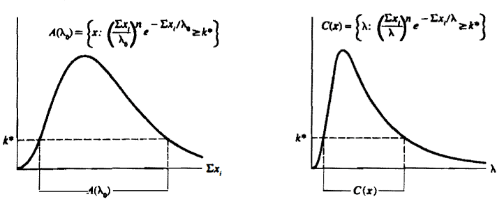
In previous section we saw that a pivot, $Q$, leads to a confidence set of the form (9.2.13), that is
$$
C(\mathbf{x})=\left{\theta_0: a \leq Q\left(\mathbf{x}, \theta_0\right) \leq b\right} .
$$
If, for every $\mathbf{x}$, the function $Q(\mathbf{x}, \theta)$ is a monotone function of $\theta$, then the confidence set $C(\mathbf{x})$ is guaranteed to be an interval. The pivots that we have seen so far, which were mainly constructed using location and scale transformations, resulted in monotone $Q$ functions and, hence, confidence intervals.

In this section we work with another pivot, one that is totally general and, with minor assumptions, will guarantee an interval.

If in doubt, or in a strange situation, we would recommend constructing a confidence set based on inverting an LRT, if possible. Such a set, although not guaranteed to be optimal, will never be very bad. However, in some cases such a tactic is too difficult, either analytically or computationally; inversion of the acceptance region can sometimes be quite a chore. If the method of this section can be applied, it is rather straightforward to implement and will usually produce a set that is reasonable.
To illustrate the type of trouble that could arise from the test inversion method, without extra conditions on the exact types of acceptance regions used, consider the following example, which illustrates one of the early methods of constructing confidence sets for a binomial success probability.

Example 9.2.11 (Shortest length binomial set) Sterne (1954) proposed the following method for constructing binomial confidence sets, a method that produces a set with the shortest length. Given $\alpha$, for each value of $p$ find the size $\alpha$ acceptance region composed of the most probable $x$ values. That is, for each $p$, order the $x=$ $0, \ldots, n$ values from the most probable to the least probable and put values into the acceptance region $A(p)$ until it has probability $1-\alpha$. Then use (9.2.1) to invert these acceptance regions to get a $1-\alpha$ confidence set, which Sterne claimed had length optimality properties.

To see the unexpected problems with this seemingly reasonable construction, consider a small example. Let $X \sim \operatorname{binomial}(3, p)$ and use confidence coefficient $1-\alpha=$ 442. Table 9.2.2 gives the acceptance regions obtained by the Sterne construction and the confidence sets derived by inverting this family of tests.

Surprisingly, the confidence set is not a confidence interval. This seemingly reasonable construction has led us to an unreasonable procedure. The blame is to be put on the pmf, as it does not behave as we expect. (See Exercise 9.18.)

统计代写|统计推断代考Statistical Inference代写|Bayesian Intervals

Thus far, when describing the interactions between the confidence interval and the parameter, we have carefully said that the interval covers the parameter, not that the parameter is inside the interval. This was done on purpose. We wanted to stress that the random quantity is the interval, not the parameter. Therefore, we tried to make the action verbs apply to the interval and not the parameter.

In Example 9.2.15 we saw that if $y_0=\sum_{i=1}^{10} x_i=6$, then a $90 \%$ confidence interval for $\lambda$ is $.262 \leq \lambda \leq 1.184$. It is tempting to say (and many experimenters do) that “the probability is $90 \%$ that $\lambda$ is in the interval $[.262,1.184] . “$ Within classical statistics, however, such a statement is invalid since the parameter is assumed fixed. Formally, the interval $[.262,1.184]$ is one of the possible realized values of the random interval $\left[\frac{1}{2 n} \chi_{2 Y, .95}^2, \frac{1}{2 n} \chi_{2(Y+1), .05}^2\right]$ and, since the parameter. $\lambda$ does not move, $\lambda$ is in the realized interval $[.262,1.184]$ with probability either 0 or 1 . When we say that the realized interval $[.262,1.184]$ has a $90 \%$ chance of coverage, we only mean that we know that $90 \%$ of the sample points of the random interval cover the true parameter.

In contrast, the Bayesian setup allows us to say that $\lambda$ is inside $[.262,1.184]$ with some probability, not 0 or 1 . This is because, under the Bayesian model, $\lambda$ is a random variable with a probability distribution. All Bayesian claims of coverage are made with respect to the posterior distribution of the parameter.

To keep the distinction between Bayesian and classical sets clear, since the sets make quite different probability assessments, the Bayesian set estimates are referred to as credible sets rather than confidence sets.

Thus, if $\pi(\theta \mid \mathbf{x})$ is the posterior distribution of $\theta$ given $\mathbf{X}=\mathbf{x}$, then for any set $A \subset \Theta$, the credible probability of $A$ is
$$
P(\theta \in A \mid \mathbf{x})=\int_A \pi(\theta \mid \mathbf{x}) d \theta,
$$
and $A$ is a credible set for $\theta$. If $\pi(\theta \mid \mathbf{x})$ is a pmf, we replace integrals with sums in the above expressions.

统计推断代写

统计代写|统计推断代考Statistical Inference代写|Pivoting the GDF

在上一节中，我们看到枢轴$Q$导致了一个形式(9.2.13)的置信集，即
$ $
C(\mathbf{x})=\left{\theta_0: a \leq Q\left(\mathbf{x}， \theta_0\右)\leq b\右}。
$ $
如果对于每一个$\mathbf{x}$，函数$Q(\mathbf{x}， \theta)$是$\theta$的单调函数，那么置信集$C(\mathbf{x})$保证是一个区间。到目前为止，我们所看到的枢轴，主要是使用位置和尺度转换构建的，导致单调的$Q$函数，因此，置信区间。

在本节中，我们将使用另一个支点，这个支点是完全通用的，并且具有较小的假设，将保证一个区间。

如果有疑问，或者在一个奇怪的情况下，我们建议在可能的情况下，基于反转LRT构造一个置信集。这样的集合，虽然不能保证是最优的，但绝不会是非常糟糕的。然而，在某些情况下，这种策略无论是在分析上还是在计算上都过于困难;接受区域的反转有时会很麻烦。如果可以应用本节的方法，则实现起来相当简单，并且通常会产生一个合理的集合。
为了说明测试反演方法可能产生的问题类型，而不需要对所使用的接受区域的确切类型附加条件，请考虑以下示例，该示例说明了为二项成功概率构建置信集的早期方法之一。

例9.2.11(最短长度二项集)Sterne(1954)提出了构造二项置信集的如下方法，该方法产生长度最短的集。给定$\alpha$，对于$p$的每个值，找出由最可能的$x$值组成的$\alpha$可接受区域的大小。也就是说，对于每个$p$，将$x=$ 0， $ ldots， $ n$的值从最可能到最不可能排序，并将值放入可接受区域$A(p)$，直到它的概率为$1- $ α $。然后使用(9.2.1)来反转这些接受区域，以得到一个$1-\alpha$置信集，Sterne声称它具有长度最优性。

要了解这个看似合理的结构所带来的意想不到的问题，请考虑一个小示例。设$X \sim \operatorname{binomial}(3, p)$，并使用置信系数$1-\alpha=$ 442。表9.2.2给出了由Sterne构造得到的可接受区域和由该检验族的反求得到的置信集。

令人惊讶的是，这个置信集不是一个置信区间。这种看似合理的构造导致了不合理的程序。这应该归咎于基金会，因为它的行为不像我们所期望的那样。(参见练习9.18。)

统计代写|统计推断代考Statistical Inference代写|Bayesian Intervals

到目前为止，在描述置信区间和参数之间的相互作用时，我们已经小心地说过区间覆盖了参数，而不是参数在区间内。这是故意的。我们要强调的是随机量是区间，而不是参数。因此，我们试图使动作动词适用于间隔而不是参数。

在例9.2.15中，我们看到如果$y_0=\sum_{i=1}^{10} x_i=6$，那么$\lambda$的$90 \%$置信区间是$.262 \leq \lambda \leq 1.184$。人们很容易说(许多实验者也这么说)“$\lambda$在区间$[.262,1.184] . “$内的概率是$90 \%$”，然而，在经典统计中，这样的说法是无效的，因为参数是假定固定的。形式上，区间$[.262,1.184]$是随机区间$\left[\frac{1}{2 n} \chi_{2 Y, .95}^2, \frac{1}{2 n} \chi_{2(Y+1), .05}^2\right]$和的可能实现值之一，因为参数。$\lambda$不移动，$\lambda$在实现区间$[.262,1.184]$内，概率为0或1。当我们说实现区间$[.262,1.184]$有$90 \%$的覆盖机会时，我们只是说我们知道该随机区间的样本点$90 \%$覆盖了真实参数。

相反，贝叶斯设置允许我们说$\lambda$以某种概率在$[.262,1.184]$内，而不是0或1。这是因为，在贝叶斯模型下，$\lambda$是一个具有概率分布的随机变量。所有关于覆盖率的贝叶斯声明都是根据参数的后验分布作出的。

为了明确贝叶斯集和经典集之间的区别，由于这些集进行的概率评估非常不同，因此贝叶斯集估计被称为可信集而不是置信集。

因此，如果$\pi(\theta \mid \mathbf{x})$是给定$\mathbf{X}=\mathbf{x}$的$\theta$的后验分布，则对于任意集$A \subset \Theta$, $A$的可信概率为
$$
P(\theta \in A \mid \mathbf{x})=\int_A \pi(\theta \mid \mathbf{x}) d \theta,
$$
$A$是$\theta$的可靠集合。如果$\pi(\theta \mid \mathbf{x})$是一个pmf，我们将上述表达式中的积分替换为和。

统计代写|统计推断代考Statistical Inference代写 请认准exambang™. exambang™为您的留学生涯保驾护航。

微观经济学代写

微观经济学是主流经济学的一个分支，研究个人和企业在做出有关稀缺资源分配的决策时的行为以及这些个人和企业之间的相互作用。my-assignmentexpert™ 为您的留学生涯保驾护航 在数学Mathematics作业代写方面已经树立了自己的口碑, 保证靠谱, 高质且原创的数学Mathematics代写服务。我们的专家在图论代写Graph Theory代写方面经验极为丰富，各种图论代写Graph Theory相关的作业也就用不着 说。

线性代数代写

线性代数是数学的一个分支，涉及线性方程，如：线性图，如：以及它们在向量空间和通过矩阵的表示。线性代数是几乎所有数学领域的核心。

博弈论代写

现代博弈论始于约翰-冯-诺伊曼（John von Neumann）提出的两人零和博弈中的混合策略均衡的观点及其证明。冯-诺依曼的原始证明使用了关于连续映射到紧凑凸集的布劳威尔定点定理，这成为博弈论和数学经济学的标准方法。在他的论文之后，1944年，他与奥斯卡-莫根斯特恩（Oskar Morgenstern）共同撰写了《游戏和经济行为理论》一书，该书考虑了几个参与者的合作游戏。这本书的第二版提供了预期效用的公理理论，使数理统计学家和经济学家能够处理不确定性下的决策。

微积分代写

微积分，最初被称为无穷小微积分或 “无穷小的微积分”，是对连续变化的数学研究，就像几何学是对形状的研究，而代数是对算术运算的概括研究一样。

它有两个主要分支，微分和积分；微分涉及瞬时变化率和曲线的斜率，而积分涉及数量的累积，以及曲线下或曲线之间的面积。这两个分支通过微积分的基本定理相互联系，它们利用了无限序列和无限级数收敛到一个明确定义的极限的基本概念 。

计量经济学代写

什么是计量经济学？
计量经济学是统计学和数学模型的定量应用，使用数据来发展理论或测试经济学中的现有假设，并根据历史数据预测未来趋势。它对现实世界的数据进行统计试验，然后将结果与被测试的理论进行比较和对比。

根据你是对测试现有理论感兴趣，还是对利用现有数据在这些观察的基础上提出新的假设感兴趣，计量经济学可以细分为两大类：理论和应用。那些经常从事这种实践的人通常被称为计量经济学家。

Matlab代写

MATLAB 是一种用于技术计算的高性能语言。它将计算、可视化和编程集成在一个易于使用的环境中，其中问题和解决方案以熟悉的数学符号表示。典型用途包括：数学和计算算法开发建模、仿真和原型制作数据分析、探索和可视化科学和工程图形应用程序开发，包括图形用户界面构建MATLAB 是一个交互式系统，其基本数据元素是一个不需要维度的数组。这使您可以解决许多技术计算问题，尤其是那些具有矩阵和向量公式的问题，而只需用 C 或 Fortran 等标量非交互式语言编写程序所需的时间的一小部分。MATLAB 名称代表矩阵实验室。MATLAB 最初的编写目的是提供对由 LINPACK 和 EISPACK 项目开发的矩阵软件的轻松访问，这两个项目共同代表了矩阵计算软件的最新技术。MATLAB 经过多年的发展，得到了许多用户的投入。在大学环境中，它是数学、工程和科学入门和高级课程的标准教学工具。在工业领域，MATLAB 是高效研究、开发和分析的首选工具。MATLAB 具有一系列称为工具箱的特定于应用程序的解决方案。对于大多数 MATLAB 用户来说非常重要，工具箱允许您学习和应用专业技术。工具箱是 MATLAB 函数（M 文件）的综合集合，可扩展 MATLAB 环境以解决特定类别的问题。可用工具箱的领域包括信号处理、控制系统、神经网络、模糊逻辑、小波、仿真等。