如果你也在 怎样代写统计推断Statistical Inference 这个学科遇到相关的难题，请随时右上角联系我们的24/7代写客服。统计推断Statistical Inference是利用数据分析来推断概率基础分布的属性的过程。推断性统计分析推断人口的属性，例如通过测试假设和得出估计值。假设观察到的数据集是从一个更大的群体中抽出的。

统计推断Statistical Inference（可以与描述性统计进行对比。描述性统计只关注观察到的数据的属性，它并不依赖于数据来自一个更大的群体的假设。在机器学习中，推理一词有时被用来代替 “通过评估一个已经训练好的模型来进行预测”；在这种情况下，推断模型的属性被称为训练或学习（而不是推理），而使用模型进行预测被称为推理（而不是预测）；另见预测推理。

统计推断Statistical Inference代写，免费提交作业要求， 满意后付款，成绩80\%以下全额退款，安全省心无顾虑。专业硕 博写手团队，所有订单可靠准时，保证 100% 原创。最高质量的统计推断Statistical Inference作业代写，服务覆盖北美、欧洲、澳洲等 国家。 在代写价格方面，考虑到同学们的经济条件，在保障代写质量的前提下，我们为客户提供最合理的价格。 由于作业种类很多，同时其中的大部分作业在字数上都没有具体要求，因此统计推断Statistical Inference作业代写的价格不固定。通常在专家查看完作业要求之后会给出报价。作业难度和截止日期对价格也有很大的影响。

同学们在留学期间，都对各式各样的作业考试很是头疼，如果你无从下手，不如考虑my-assignmentexpert™！

my-assignmentexpert™提供最专业的一站式服务：Essay代写，Dissertation代写，Assignment代写，Paper代写，Proposal代写，Proposal代写，Literature Review代写，Online Course，Exam代考等等。my-assignmentexpert™专注为留学生提供Essay代写服务，拥有各个专业的博硕教师团队帮您代写，免费修改及辅导，保证成果完成的效率和质量。同时有多家检测平台帐号，包括Turnitin高级账户，检测论文不会留痕，写好后检测修改，放心可靠，经得起任何考验！

统计代写|统计推断代考Statistical Inference代写|Multiple Hypotheses

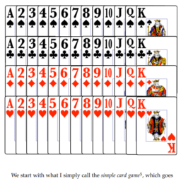
We start this section with an example.
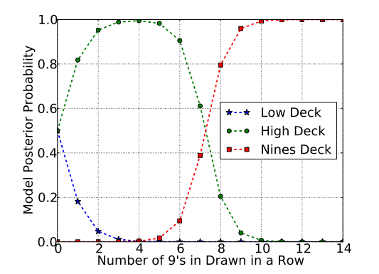
EXAMPLE 4.2 What is the probability that you are holding one of either the High or the Low Deck having drawn five g’s in a row from that deck?
We have observed the following data:
$$
\text { data } \equiv\left{\begin{array}{l}
\text { “We’ve drawn one card, and it is a 9, replaced } \
\text { and reshuffled, redrawn and observed another } \
\text { 9, repeated this procedure and observed three } \
\text { more 9’s, for a total of five 9’s in a row.” }
\end{array}\right.
$$
Technically, drawing 5 9’s in a row should give us really strong confidence that you are drawing from the High Deck, because we would have
I Specify the prior probabilities for the models being considered
$$
\begin{gathered}
P(H)=0.5 \
P(L)=0.5
\end{gathered}
$$
2 Write the top of Bayes’ Rule for all models being considered
$$
\begin{aligned}
& P(H \mid \text { data }=5 \text { 9’s in a row }) \sim P\left(\text { data }=59^{\prime} \text { s in a row } \mid H\right) P(H) \
& P\left(L \mid \text { data }=59^{\prime} \text { s in a row }\right) \sim P\left(\text { data }=59^{\prime} \text { s in a row } \mid L\right) P(L) \
&
\end{aligned}
$$
3 Put in the likelihood and prior values
$$
\begin{aligned}
P\left(H \mid \text { data }=59^{\prime} \text { s in a row }\right) & \sim \underbrace{\frac{9}{55} \times \frac{9}{55} \cdots \frac{9}{55}}_{5 \text { times }} \times P(H) \
& \sim\left(\frac{9}{55}\right)^5 \times 0.5 \
& =0.0000587 \
P\left(L \mid \text { data }=59^{\prime} \text { s in a row }\right) & \sim\left(\frac{2}{55}\right)^5 \times 0.5 \
& =0.0000000318
\end{aligned}
$$
4 Add these values for all models
$$
K=0.0000587+0.0000000318=0.0000587318
$$
5 Divide each of the values by this sum, $K$, to get the final probabilities
$$
\begin{aligned}
P(H \mid \text { data }=5 \text { g’s in a row }) & =\frac{0.0000587}{0.0000587318}=0.99946 \
P(L \mid \text { data }=5 \text { g’s in a row }) & =\frac{0.0000000318}{0.0000587318}=0.00054
\end{aligned}
$$
which is fantastically on the side of the high deck, even though we might start getting suspicious in this situation.

统计代写|统计推断代考Statistical Inference代写|Disease Testing

Let’s imagine there is a rare, one in a million, disease that is lethal but does not have many outward symptoms at first. A new test boasts $99.9 \%$ accuracy, so you go to get tested, and receive the bad news that you test positive for the disease. Should you be devastated by the news? What is the probability that you actually have the disease? We are looking at two, quite different, probabilities here. In the first case, we have the claims of the test which state that if you have the disease, the probability that the test will be positive is o.999, or, if you have the disease, test will discover that fact $99.9 \%$ of the time. In the second case we have your concern which is, if you test positive for the test, what is the probability that you have the disease. In our notation this is:
$$
\begin{aligned}
& P(\text { positive test } \mid \text { disease })=0.999 \text { (claim from test) } \
& P(\text { disease } \mid \text { positive test })=?(\text { your concern) }
\end{aligned}
$$
These two are related by Bayes’ Rule (Equation 1.14). The Bayes’ Recipe proceeds as follows
1 Specify the prior probabilities for the models being considered The models we have are simply “have the disease” and “don’t have the disease”. The prior probabilities for these two come from the prevalence of the disease in the population, before you get tested. Since this is a “one in a million” disease, we have
$$
\begin{aligned}
P(\text { disease }) & =\frac{1}{1,000,000} \
P(\text { no disease }) & =\frac{999,999}{1,000,000}
\end{aligned}
$$
2 Write the top of Bayes’ Rule for all models being considered
The top of Bayes’ Rule comes down to, given the truth of the model (i.e. either with or without the disease), what is the probability of getting the data (i.e. the positive or negative test result). This is measured by how good the test is.
$$
P(\text { positive test } \mid \text { disease })=0.999
$$
and
$$
P(\text { positive test } \mid \text { no disease })=0.001
$$
So the top of Bayes’ Rule looks for both models looks like:
$$
\begin{aligned}
P(\text { disease } \mid \text { positive test }) & \sim P(\text { positive test } \mid \text { disease }) \times P(\text { disease }) \
& \sim 0.999 \times \frac{1}{1,000,000}=9.99 \cdot 10^{-7} \
P(\text { no disease } \mid \text { positive test }) & \sim P(\text { positive test } \mid \text { no disease }) \times P(\text { no disease }) \
& \sim 0.001 \times \frac{999,999}{1,000,000}=9.99 \cdot 10^{-4}
\end{aligned}
$$
3 Add these values for all models
$$
K=9.99 \cdot 10^{-7}+9.99 \cdot 10^{-4}=0.000999999
$$
4 Divide each of the values by this sum, $K$, to get the final probabilities
$$
\begin{aligned}
P(\text { disease } \mid \text { positive test }) & =\frac{9.99 \cdot 10^{-7}}{0.000999999}=0.1 \% \
P(\text { no disease } \mid \text { positive test }) & =99.9 \%
\end{aligned}
$$

统计推断代写

统计代写|统计推断代考Statistical Inference代写|Multiple Hypotheses

我们以一个示例开始本节。例4.2你持有一张高牌或一张低牌的概率是多少?从这副牌中连续抽到5张g ?
我们观察了以下数据:
$$
\text {data} \equiv\left{\begin{array}{l}
\text{“我们已经抽了一张牌，它是一张9，替换了}\
\text{并重新洗牌，重新抽牌并观察了另一张}\
\text{9，重复这个过程并观察了三个}\
\text{更多的9，一行总共有五个9。”} < br > \{数组}\右结束。
$$
从技术上讲，连续画5个9应该给我们很强的信心，你是从高层绘图，因为我们会有
1指定被考虑的模型的先验概率
$$
\begin{gather}
P(H)=0.5 \
P(L)=0.5
\end{gather}
$$
2为所有被考虑的模型写下贝叶斯规则的顶端
$$
\begin{aligned}
&;P(H \mid \text {data}=5 \text {9′ in a row}) \sim P\left(\text {data}=59^{\prime} \text {s in a row} \mid H\right) P(H) \
&P\left(L \mid \text {data}=59^{\prime} \text {s in a row}\ mid L\right) P(L) \
&
\end{aligned}
$$
\begin{aligned}
P\left(H \mid \text {data}=59^{\prime} \text {s in a row}\right) &\ sim \ underbrace{\压裂{9}{55}\ * \压裂{9}{55}\ cdots \压裂{9}{55}}_{5 \文本{倍}}\乘以P (H) \ < br >,左(\ \ sim \压裂{9}{55}\右)^ 5 \ * 0.5 \ < br >,=0.0000587 \
P\left(L \mid \text {data}=59^{\prime} \text {s in a row}\right) &左(\ \ sim \压裂{2}{55}\右)^ 5 \ * 0.5 \ < br >,=0.0000000318
\end{aligned}
$$
4将所有模型的这些值相加
$$
K=0.0000587+0.0000000318=0.0000587318
$$
5将每个值除以这个和$K$，得到最终的概率
$$
\begin{aligned}
P(H \mid \text {data}=5 \text {g’s ina row}) &=\frac{0.0000587}{0.0000587318}=0.99946 \
P(L \mid \text {data}=5 \text {g’s in a row}) &=\frac{0.0000000318}{0.0000587318}=0.00054
\end{aligned}
$$
这是在高甲板的一边，尽管我们可能会开始怀疑在这种情况下。

统计代写|统计推断代考Statistical Inference代写|Disease Testing

让我们想象一下，有一种罕见的，百万分之一的致命疾病，一开始并没有很多外在症状。一种新的检测方法号称$99.9 \%$的准确性，所以你去做了检测，却得到了一个坏消息:你的检测结果呈阳性。你应该为这个消息感到震惊吗?你真的患病的概率是多少?我们现在看到的是两种完全不同的概率。在第一种情况下，我们有测试的声明声明如果你有疾病，测试呈阳性的概率是0.999，或者，如果你有疾病，测试会发现这个事实$99.9 \%$的时间。在第二种情况下，我们有你关心的是，如果你的测试呈阳性，你患病的概率是多少。在我们的符号中是:
$$
\begin{aligned}
& P(\text { positive test } \mid \text { disease })=0.999 \text { (claim from test) } \
& P(\text { disease } \mid \text { positive test })=?(\text { your concern) }
\end{aligned}
$$
这两者通过贝叶斯规则(公式1.14)联系起来。贝叶斯公式的过程如下
1 .指定所考虑的模型的先验概率。我们所拥有的模型只是“有这种疾病”和“没有这种疾病”。这两个的先验概率来自于在你接受检测之前，疾病在人群中的流行程度。由于这是“百万分之一”的疾病，我们有
$$
\begin{aligned}
P(\text { disease }) & =\frac{1}{1,000,000} \
P(\text { no disease }) & =\frac{999,999}{1,000,000}
\end{aligned}
$$
写下所有考虑的模型的贝叶斯规则的顶部
贝叶斯规则的顶部归结为，给定模型的真值(即有或没有疾病)，获得数据的概率(即阳性或阴性测试结果)是多少。这是通过测试的好坏来衡量的。
$$
P(\text { positive test } \mid \text { disease })=0.999
$$
和
$$
P(\text { positive test } \mid \text { no disease })=0.001
$$
所以两个模型的贝叶斯规则的顶部看起来是这样的
$$
\begin{aligned}
P(\text { disease } \mid \text { positive test }) & \sim P(\text { positive test } \mid \text { disease }) \times P(\text { disease }) \
& \sim 0.999 \times \frac{1}{1,000,000}=9.99 \cdot 10^{-7} \
P(\text { no disease } \mid \text { positive test }) & \sim P(\text { positive test } \mid \text { no disease }) \times P(\text { no disease }) \
& \sim 0.001 \times \frac{999,999}{1,000,000}=9.99 \cdot 10^{-4}
\end{aligned}
$$
3将所有型号的数值相加
$$
K=9.99 \cdot 10^{-7}+9.99 \cdot 10^{-4}=0.000999999
$$
4将每个值除以这个和$K$，得到最终的概率
$$
\begin{aligned}
P(\text { disease } \mid \text { positive test }) & =\frac{9.99 \cdot 10^{-7}}{0.000999999}=0.1 \% \
P(\text { no disease } \mid \text { positive test }) & =99.9 \%
\end{aligned}
$$

统计代写|统计推断代考Statistical Inference代写 请认准exambang™. exambang™为您的留学生涯保驾护航。

微观经济学代写

微观经济学是主流经济学的一个分支，研究个人和企业在做出有关稀缺资源分配的决策时的行为以及这些个人和企业之间的相互作用。my-assignmentexpert™ 为您的留学生涯保驾护航 在数学Mathematics作业代写方面已经树立了自己的口碑, 保证靠谱, 高质且原创的数学Mathematics代写服务。我们的专家在图论代写Graph Theory代写方面经验极为丰富，各种图论代写Graph Theory相关的作业也就用不着 说。

线性代数代写

线性代数是数学的一个分支，涉及线性方程，如：线性图，如：以及它们在向量空间和通过矩阵的表示。线性代数是几乎所有数学领域的核心。

博弈论代写

现代博弈论始于约翰-冯-诺伊曼（John von Neumann）提出的两人零和博弈中的混合策略均衡的观点及其证明。冯-诺依曼的原始证明使用了关于连续映射到紧凑凸集的布劳威尔定点定理，这成为博弈论和数学经济学的标准方法。在他的论文之后，1944年，他与奥斯卡-莫根斯特恩（Oskar Morgenstern）共同撰写了《游戏和经济行为理论》一书，该书考虑了几个参与者的合作游戏。这本书的第二版提供了预期效用的公理理论，使数理统计学家和经济学家能够处理不确定性下的决策。

微积分代写

微积分，最初被称为无穷小微积分或 “无穷小的微积分”，是对连续变化的数学研究，就像几何学是对形状的研究，而代数是对算术运算的概括研究一样。

它有两个主要分支，微分和积分；微分涉及瞬时变化率和曲线的斜率，而积分涉及数量的累积，以及曲线下或曲线之间的面积。这两个分支通过微积分的基本定理相互联系，它们利用了无限序列和无限级数收敛到一个明确定义的极限的基本概念 。

计量经济学代写

什么是计量经济学？
计量经济学是统计学和数学模型的定量应用，使用数据来发展理论或测试经济学中的现有假设，并根据历史数据预测未来趋势。它对现实世界的数据进行统计试验，然后将结果与被测试的理论进行比较和对比。

根据你是对测试现有理论感兴趣，还是对利用现有数据在这些观察的基础上提出新的假设感兴趣，计量经济学可以细分为两大类：理论和应用。那些经常从事这种实践的人通常被称为计量经济学家。

Matlab代写

MATLAB 是一种用于技术计算的高性能语言。它将计算、可视化和编程集成在一个易于使用的环境中，其中问题和解决方案以熟悉的数学符号表示。典型用途包括：数学和计算算法开发建模、仿真和原型制作数据分析、探索和可视化科学和工程图形应用程序开发，包括图形用户界面构建MATLAB 是一个交互式系统，其基本数据元素是一个不需要维度的数组。这使您可以解决许多技术计算问题，尤其是那些具有矩阵和向量公式的问题，而只需用 C 或 Fortran 等标量非交互式语言编写程序所需的时间的一小部分。MATLAB 名称代表矩阵实验室。MATLAB 最初的编写目的是提供对由 LINPACK 和 EISPACK 项目开发的矩阵软件的轻松访问，这两个项目共同代表了矩阵计算软件的最新技术。MATLAB 经过多年的发展，得到了许多用户的投入。在大学环境中，它是数学、工程和科学入门和高级课程的标准教学工具。在工业领域，MATLAB 是高效研究、开发和分析的首选工具。MATLAB 具有一系列称为工具箱的特定于应用程序的解决方案。对于大多数 MATLAB 用户来说非常重要，工具箱允许您学习和应用专业技术。工具箱是 MATLAB 函数（M 文件）的综合集合，可扩展 MATLAB 环境以解决特定类别的问题。可用工具箱的领域包括信号处理、控制系统、神经网络、模糊逻辑、小波、仿真等。