数学代写|Function fitting and interpolation 凸优化代考
凸优化代写
6.5.1 Function families
We consider a family of functions $f_{1}, \ldots, f_{n}: \mathbf{R}^{k} \rightarrow \mathbf{R}$, with common domain $\operatorname{dom} f_{i}=D .$ With each $x \in \mathbf{R}^{n}$ we associate the function $f: \mathbf{R}^{k} \rightarrow \mathbf{R}$ given by
$$
f(u)=x_{1} f_{1}(u)+\cdots+x_{n} f_{n}(u)
$$
with $\operatorname{dom} f=D$. The family $\left{f_{1}, \ldots, f_{n}\right}$ is sometimes called the set of basis functions (for the fitting problem) even when the functions are not independent. The vector $x \in \mathbf{R}^{n}$, which parametrizes the subspace of functions, is our optimization variable, and is sometimes called the coefficient vector. The basis functions generate a subspace $\mathcal{F}$ of functions on $D$.
In many applications the basis functions are specially chosen, using prior knowledge or experience, in order to reasonably model functions of interest with the finite-dimensional subspace of functions. In other cases, more generic function families are used. We describe a few of these below.
Polynomials
One common subspace of functions on $\mathbf{R}$ consists of polynomials of degree less than $n$. The simplest basis consists of the powers, i.e., $f_{i}(t)=t^{i-1}, i=1, \ldots, n$. In many applications, the same subspace is described using a different basis, for example, a set of polynomials $f_{1}, \ldots, f_{n}$, of degree less than $n$, that are orthonormal with respect to some positive function (or measure) $\phi: \mathbf{R}^{n} \rightarrow \mathbf{R}{+}$, i.e., $$ \int f{i}(t) f_{j}(t) \phi(t) d t= \begin{cases}1 & i=j \ 0 & i \neq j\end{cases}
$$
Another common basis for polynomials is the Lagrange basis $f_{1}, \ldots, f_{n}$ associated with distinct points $t_{1}, \ldots, t_{n}$, which satisfy
$$
f_{i}\left(t_{j}\right)= \begin{cases}1 & i=j \ 0 & i \neq j\end{cases}
$$
We can also consider polynomials on $\mathbf{R}^{k}$, with a maximum total degree, or a maximum degree for each variable.
As a related example, we have trigonometric polynomials of degree less than $n$, with basis
$$
\sin k t, \quad k=1, \ldots, n-1, \quad \cos k t, \quad k=0, \ldots, n-1
$$
Piecewise-linear functions
We start with a triangularization of the domain $D$, which means the following. We have a set of mesh or grid points $g_{1}, \ldots, g_{n} \in \mathbf{R}^{k}$, and a partition of $D$ into a set of simplexes:
$$
D=S_{1} \cup \cdots \cup S_{m}, \quad \operatorname{int}\left(S_{i} \cap S_{j}\right)=\emptyset \text { for } i \neq j
$$
$u_{2}$ of two variables, on the unit square.
Figure $6.17$ A piecewise-linear function of two variables, on the unit square. The triangulation consists of 98 simplexes, and a uniform grid of 64 points in the unit square.
Each simplex is the convex hull of $k+1$ grid points, and we require that each grid point is a vertex of any simplex it lies in.
Given a triangularization, we can construct a piecewise-linear (or more precisely, piecewise-affine) function $f$ by assigning function values $f\left(g_{i}\right)=x_{i}$ to the grid points, and then extending the function affinely on each simplex. The function $f$ can be expressed as $(6.17)$ where the basis functions $f_{i}$ are affine on each simplex and are defined by the conditions
$$
f_{i}\left(g_{j}\right)= \begin{cases}1 & i=j \ 0 & i \neq j\end{cases}
$$
By construction, such a function is continuous.
Figure $6.17$ shows an example for $k=2$.
Piecewise polynomials and splines
The idea of piecewise-affine functions on a triangulated domain is readily extended to piecewise polynomials and other functions.
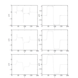
Piecewise polynomials are defined as polynomials (of some maximum degree) on each simplex of the triangulation, which are continuous, i.e., the polynomials agree at the boundaries between simplexes. By further restricting the piecewise polynomials to have continuous derivatives up to a certain order, we can define various classes of spline functions. Figure $6.18$ shows an example of a cubic spline, i.e., a piecewise polynomial of degree 3 on $\mathbf{R}$, with continuous first and second derivatives.
凸优化代考
6.5.1 Function families
We consider a family of functions $f_{1}, \ldots, f_{n}: \mathbf{R}^{k} \rightarrow \mathbf{R}$, with common domain $\operatorname{dom} f_{i}=D .$ With each $x \in \mathbf{R}^{n}$ we associate the function $f: \mathbf{R}^{k} \rightarrow \mathbf{R}$ given by
$$
f(u)=x_{1} f_{1}(u)+\cdots+x_{n} f_{n}(u)
$$
with $\operatorname{dom} f=D$. The family $\left{f_{1}, \ldots, f_{n}\right}$ is sometimes called the set of basis functions (for the fitting problem) even when the functions are not independent. The vector $x \in \mathbf{R}^{n}$, which parametrizes the subspace of functions, is our optimization variable, and is sometimes called the coefficient vector. The basis functions generate a subspace $\mathcal{F}$ of functions on $D$.
In many applications the basis functions are specially chosen, using prior knowledge or experience, in order to reasonably model functions of interest with the finite-dimensional subspace of functions. In other cases, more generic function families are used. We describe a few of these below.
Polynomials
One common subspace of functions on $\mathbf{R}$ consists of polynomials of degree less than $n$. The simplest basis consists of the powers, i.e., $f_{i}(t)=t^{i-1}, i=1, \ldots, n$. In many applications, the same subspace is described using a different basis, for example, a set of polynomials $f_{1}, \ldots, f_{n}$, of degree less than $n$, that are orthonormal with respect to some positive function (or measure) $\phi: \mathbf{R}^{n} \rightarrow \mathbf{R}{+}$, i.e., $$ \int f{i}(t) f_{j}(t) \phi(t) d t= \begin{cases}1 & i=j \ 0 & i \neq j\end{cases}
$$
Another common basis for polynomials is the Lagrange basis $f_{1}, \ldots, f_{n}$ associated with distinct points $t_{1}, \ldots, t_{n}$, which satisfy
$$
f_{i}\left(t_{j}\right)= \begin{cases}1 & i=j \ 0 & i \neq j\end{cases}
$$
We can also consider polynomials on $\mathbf{R}^{k}$, with a maximum total degree, or a maximum degree for each variable.
As a related example, we have trigonometric polynomials of degree less than $n$, with basis
$$
\sin k t, \quad k=1, \ldots, n-1, \quad \cos k t, \quad k=0, \ldots, n-1
$$
Piecewise-linear functions
We start with a triangularization of the domain $D$, which means the following. We have a set of mesh or grid points $g_{1}, \ldots, g_{n} \in \mathbf{R}^{k}$, and a partition of $D$ into a set of simplexes:
$$
D=S_{1} \cup \cdots \cup S_{m}, \quad \operatorname{int}\left(S_{i} \cap S_{j}\right)=\emptyset \text { for } i \neq j
$$
$u_{2}$ of two variables, on the unit square.
Figure $6.17$ A piecewise-linear function of two variables, on the unit square. The triangulation consists of 98 simplexes, and a uniform grid of 64 points in the unit square.
Each simplex is the convex hull of $k+1$ grid points, and we require that each grid point is a vertex of any simplex it lies in.
Given a triangularization, we can construct a piecewise-linear (or more precisely, piecewise-affine) function $f$ by assigning function values $f\left(g_{i}\right)=x_{i}$ to the grid points, and then extending the function affinely on each simplex. The function $f$ can be expressed as $(6.17)$ where the basis functions $f_{i}$ are affine on each simplex and are defined by the conditions
$$
f_{i}\left(g_{j}\right)= \begin{cases}1 & i=j \ 0 & i \neq j\end{cases}
$$
By construction, such a function is continuous.
Figure $6.17$ shows an example for $k=2$.
Piecewise polynomials and splines
The idea of piecewise-affine functions on a triangulated domain is readily extended to piecewise polynomials and other functions.
Piecewise polynomials are defined as polynomials (of some maximum degree) on each simplex of the triangulation, which are continuous, i.e., the polynomials agree at the boundaries between simplexes. By further restricting the piecewise polynomials to have continuous derivatives up to a certain order, we can define various classes of spline functions. Figure $6.18$ shows an example of a cubic spline, i.e., a piecewise polynomial of degree 3 on $\mathbf{R}$, with continuous first and second derivatives.

数学代写| Chebyshev polynomials 数值分析代考 请认准UprivateTA™. UprivateTA™为您的留学生涯保驾护航。
时间序列分析代写
统计作业代写
随机过程代写
随机过程,是依赖于参数的一组随机变量的全体,参数通常是时间。 随机变量是随机现象的数量表现,其取值随着偶然因素的影响而改变。 例如,某商店在从时间t0到时间tK这段时间内接待顾客的人数,就是依赖于时间t的一组随机变量,即随机过程