如果你也在 怎样代写运筹学Operations Research这个学科遇到相关的难题,请随时右上角联系我们的24/7代写客服。假设检验Hypothesis是假设检验是统计学中的一种行为,分析者据此检验有关人口参数的假设。分析师采用的方法取决于所用数据的性质和分析的原因。假设检验是通过使用样本数据来评估假设的合理性。
运筹学(Operation)是近代应用数学的一个分支。它把具体的问题进行数学抽象,然后用像是统计学、数学模型和算法等方法加以解决,以此来寻找复杂问题中的最佳或近似最佳的解答。
二战中运筹学的应用
在二战时期,作战研究被定义为 “一种科学方法,为执行部门提供有关其控制的行动的决策的量化依据”。它的其他名称包括作战分析(英国国防部从1962年开始)和定量管理。
在第二次世界大战期间,英国有近1000名男女从事作战研究。大约有200名作战研究科学家为英国军队工作。
帕特里克-布莱克特在战争期间为几个不同的组织工作。战争初期,在为皇家飞机研究所(RAE)工作时,他建立了一个被称为 “马戏团 “的团队,帮助减少了击落一架敌机所需的防空炮弹数量,从不列颠战役开始时的平均超过20,000发减少到1941年的4,000发。
my-assignmentexpert™ 运筹学Operations Research作业代写,免费提交作业要求, 满意后付款,成绩80\%以下全额退款,安全省心无顾虑。专业硕 博写手团队,所有订单可靠准时,保证 100% 原创。my-assignmentexpert™, 最高质量的运筹学Operations Research作业代写,服务覆盖北美、欧洲、澳洲等 国家。 在代写价格方面,考虑到同学们的经济条件,在保障代写质量的前提下,我们为客户提供最合理的价格。 由于统计Statistics作业种类很多,同时其中的大部分作业在字数上都没有具体要求,因此运筹学Operations Research作业代写的价格不固定。通常在经济学专家查看完作业要求之后会给出报价。作业难度和截止日期对价格也有很大的影响。
想知道您作业确定的价格吗? 免费下单以相关学科的专家能了解具体的要求之后在1-3个小时就提出价格。专家的 报价比上列的价格能便宜好几倍。
my-assignmentexpert™ 为您的留学生涯保驾护航 在运筹学Operations Research作业代写方面已经树立了自己的口碑, 保证靠谱, 高质且原创的应用数学applied math代写服务。我们的专家在运筹学Operations Research代写方面经验极为丰富,各种运筹学Operations Research相关的作业也就用不着 说。
我们提供的假设检验Hypothesis及其相关学科的代写,服务范围广, 其中包括但不限于:
- 商业分析 Business Analysis
- 计算机科学 Computer Science
- 数据挖掘/数据科学/大数据 Data Mining / Data Science / Big Data
- 决策分析 Decision Analytics
- 金融工程 Financial Engineering
- 数据预测 Data Forecasting
- 博弈论 Game Theory
- 地理/地理信息科学 Geography/Geographic Information Science
- 图论 Graph Theory
- 工业工程 Industrial Engineering
- 库存控制 Inventory control
- 数学建模 Mathematical Modeling
- 数学优化 Mathematical Optimization
- 概率和统计 Probability and statistics
- 排队论 Queueing theory
- 社交网络/交通预测模型 Social network/traffic prediction modeling
- 随机过程 Stochastic processes
- 供应链管理 Supply chain management
运筹学代写
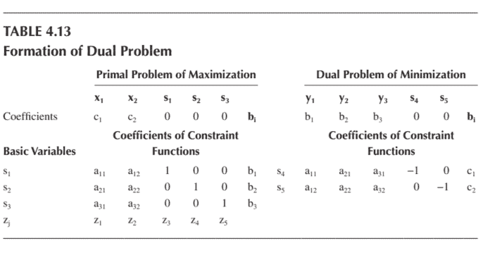
数学代写|运筹学作业代写OPERATIONS RESEARCH代考|ConstRuCtion of dual PRoblem
The construction of a dual problem from a primal problem should follow the following steps:
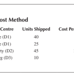
- RHS values of constraint functions of primal problem are the objective function coefficients of dual problem, i.e. $b_{i}$ of primal becomes $c_{j}$ of dual. Similarly, $c_{\mathrm{j}}$ of primal would become $b_{\mathrm{i}}$ of dual. As there are only two such coefficients in above primal problem, so in the dual problem, instead of three RHS values of three constraints, only two constraints would be created with coefficients of objective functions $\left(c_{j}\right)$ as right and side values $\left(b_{i}\right)$ of the dual problem.
- Maximization primal problem would become minimization dual problem and vice versa. The reason for this is very simple. The new solution as indicated by solving dual problem would be feasible if the primal problem is optimal. Thus, the optimality of primal corresponds to the feasibility of dual. As a result, the optimal value of $Z$ in primal is minimum feasible in dual, so it should be minimized in the case of maximization of primal.
- Number of decision variables in the primal problem would be the same as the number of constraints in the dual problem. In this case, there are two decision variables in the primal problem, i.e. $x_{1}$ and $x_{2}$. Thus, the dual problem will have two constraints instead of three as were in primal.
- Number of constraints in the primal problem is the same as the number of decision variables in the dual problem. In the primal problem, this case has three constraint functions. Thus, a dual problem will have three variables called dual variables in the objective function instead of two. Dual variables are represented as $\mathrm{y}{1}, \mathrm{y}{2}$ and $\mathrm{y}{3}$ pertaining to each of the constraints. In the above illustration, $\mathrm{y}{1}$ represents accessibility constraint, $\mathrm{y}{2}$ population density constraint and $\mathrm{y}{3}$ represents median income constraint.
- The inequalities would be reversed, i.e. as dual is opposite and mirror of primal, less than inequality in the primal would convert to greater than equal to in the dual.
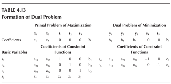
数学代写|运筹学作业代写OPERATIONS RESEARCH代考|RelationshiP betWeen PRimal and dual PRoblem
It is important to note that in simplex table of primal problem:
- There are three constraint equations, whereas the dual problem has only two.
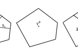
- $s_{1}, s_{2}$ and $s_{3}$ are slack variables as inequalities were of less than or equal to, whereas in dual, $\mathrm{s}{4}$ and $\mathrm{s}{5}$ are surplus variables as inequalities were greater than or equal to.
- Relationship between basic and non-basic variables of primal and dual: As per definition, variables with zero value are termed as non-basic, whereas those with some value in optimal solution are termed as basic
variables. Also, according to duality theory, which is mirror image of primal, variables of dual are complementary to primal, i.e. basic variables of primal would be considered as non-basic of dual, whereas non-basic of primal would be basic of dual. The initial solution, as shown in the previous chapter, while calculating LPP by using the Simplex method showed that $\mathrm{x}{1}$ and $\mathrm{x}{2}$ are non-basic variables. In the dual problem, $\mathrm{s}{4}$ and $\mathrm{s}{5}$ i.e. surplus variables are basic so coefficients of decision variables $\left(x_{1}\right.$ and $\left.x_{2}\right)$ in $z_{j}$ row of primal $\left(\mathrm{z}{1}\right.$ and $\left.\mathrm{z}{2}\right)$ gives corresponding values of surplus variables of dual i.e. $s_{4}$ and $s_{5}$. This is because, as indicated in iterations 0 of simplex tableau, $\mathrm{z}{\mathrm{j}}$ row contains coefficients of decision variables $\mathrm{x}{1}$ and $\mathrm{x}{2}$ in the form of $z{1}$ and $z_{2}$, respectively, and coefficients of slack variables $s_{1}, s_{2}$ and $s_{3}$ in the form $z_{3}, z_{4}$ and $z_{5}$, respectively. Similarly, slack variables $s_{1}, s_{2}$ and $s_{3}$ in initial primal solution are basic which would transform into non-basic in initial dual solution, i.e. $\mathrm{y}{1}, \mathrm{y}{2}$ and $\mathrm{y}{3}$. So coefficients of slack variables in $\mathrm{z}{\mathrm{j}}$ row of primal $\left(\mathrm{z}{3}, \mathrm{z}{4}\right.$ and $\left.\mathrm{z}_{5}\right)$ would correspond to objective function values of the dual problem. This is because a slack variable represents the amount of resource consumed or remaining resource. For instance, if out of a maximum of 100 hours of production time, manufacturing of one unit takes 3 hours, so the remaining 97 hours is represented by a slack variable. It can also be seen as amount of production time consumed indicating the level of activity, i.e. a decision variable. Hence, it is safe to assume that slack variables of primal correspond to decision variables of dual. This transformation is shown in Table 4.14.
- Feasibility of dual: Furthermore, as indicated in the above discussion, values of surplus variables $\mathrm{s}{4}$ and $\mathrm{s}{5}$ are represented by coefficients of decision variables in $\mathrm{z}_{\mathrm{j}}$ row of primal. For dual to be feasible, these surplus variables should fulfil criteria of non-negativity, i.e. they must be either zero or greater than zero. So if these coefficients in primal are positive, then it can be inferred that dual is feasible.
数学代写|运筹学作业代写OPERATIONS RESEARCH代考|dual PRoblem of standaRd lPP
The above-shown model of sales maximization is a standard form of a linear programming problem. A maximization problem involving functional constraints with only less than or equal to $(\leq)$ inequalities is considered to be a standard form. As discussed in Chapter 3 , on the simplex method, only slack variables are added to constraint equations to convert inequalities to equalities. Furthermore, these slack variables representing the amount of remaining resources should fulfil criteria of non-negativity. On the other hand, a minimization problem cannot be constructed by definition without greater than equal to $(\geq)$ or equal to $(=)$ inequalities. These inequalities imply a minimum value that an activity can achieve optimally. In addition, surplus variables are subtracted from the constraint equations to make lefthand side equal to RHS and apply the simplex method. But when decision variables are assumed as non-basic variables, then these surplus variables violates criteria of non-negativity. To rectify, this artificial variable is added to the equation, the value of which would be greater than surplus variables. Due to the involvement of artificial variable because of the mentioned reason, the LPP form is considered as non-standard.Maximize $Z=80 x_{1}+40 x_{2}$
Constraint $1: 9 x_{1}+4 x_{2} \leq 14$
Constraint $2: 2 x_{1}+7 x_{2} \leq 10$
运筹学代考
数学代写|运筹学作业代写OPERATIONS RESEARCH代考|CONSTRUCTION OF DUAL PROBLEM
从原始问题构造对偶问题应遵循以下步骤:
- 原始问题的约束函数的 RHS 值是对偶问题的目标函数系数,即b一世原始的变成Cj双的。相似地,Cj原始的会变成b一世双的。由于上述原始问题中只有两个这样的系数,所以在对偶问题中,不是三个约束的三个 RHS 值,而是用目标函数的系数创建两个约束(Cj)作为右值和侧值(b一世)的对偶问题。
- 最大化原始问题将变成最小化对偶问题,反之亦然。原因很简单。如果原始问题是最优的,那么解决对偶问题所表明的新解决方案将是可行的。因此,原始的最优性对应于对偶的可行性。因此,最优值和in primal 在对偶中是最小可行的,所以在 primal 最大化的情况下应该最小化。
- 原始问题中决策变量的数量与对偶问题中的约束数量相同。在这种情况下,原始问题中有两个决策变量,即X1和X2. 因此,对偶问题将有两个约束,而不是原始问题中的三个约束。
- 原始问题中的约束数与对偶问题中的决策变量数相同。在原始问题中,这种情况具有三个约束函数。因此,对偶问题将在目标函数中包含三个变量,称为对偶变量,而不是两个。双变量表示为 表示收入中位数约束。
- 不等式将被反转,即由于对偶是相反的并且是原始的镜像,原始中的小于不等式将转换为对偶中的大于等于。
数学代写|运筹学作业代写OPERATIONS RESEARCH代考|RELATIONSHIP BETWEEN PRIMAL AND DUAL PROBLEM
重要的是要注意,在原始问题的单纯形表中:
- 有三个约束方程,而对偶问题只有两个。
- s1,s2和s3是松弛变量,因为不等式小于或等于,而在对偶中,$\mathrm{s} {4}一种nd\mathrm{s} {5}$ 是剩余变量,因为不等式大于或等于。
- 原始和对偶的基本变量和非基本变量之间的关系:根据定义,具有零值的变量称为非基本变量,而在最优解中具有某些值的变量称为基本变量
In the dual problem, s4 and s5 i.e. surplus variables are basic so coefficients of decision variables (x1 and x2) in zj
row of primal (z1 and z2) gives corresponding values of surplus variables of duali.e. s4 and s5. This is because, as indicated in iterations 0 of simplex tableau,zjrow contains coefficients of decision variables x1 and x2 in the form ofz1 and z2, respectively, and coefficients of slack variables s1, s2 and s3 in the form z3, z4 and z5, respectively. Similarly, slack variables s1, s2 and s3
in initial primal solution are basic which would transform into non-basic in initial dual solution, i.e. y1, y2 and y3. So coefficients of slack variables in zj row of primal (z3, z4 and z5)
同样,根据原始的镜像对偶理论,对偶的变量与原始的互补,即原始的基本变量将被认为是对偶的非基本变量,而原始的非基本变量将是对偶的基本。如上一章所示的初始解,在使用单纯形法计算 LPP 时表明
将对应于对偶问题的目标函数值。这是因为松弛变量表示消耗的资源量或剩余资源量。例如,如果在最多 100 小时的生产时间中,制造一个单元需要 3 小时,那么剩余的 97 小时由松弛变量表示。它也可以看作是表示活动水平的生产时间消耗量,即一个决策变量。因此,可以安全地假设原始的松弛变量对应于对偶的决策变量。
- 对偶的可行性:此外,如上述讨论所示,剩余变量的值 $\mathrm{s} {4}一种nd\mathrm{s} {5}一种r和r和pr和s和n吨和db和C○和FF一世C一世和n吨s○Fd和C一世s一世○nv一种r一世一种b一世和s一世n\mathrm{z}_{\mathrm{j}}$ 行原始数据。为了使对偶可行,这些剩余变量应满足非负性标准,即它们必须为零或大于零。因此,如果这些 primal 中的系数为正,则可以推断对偶是可行的。然后,可以将这些系数的值放入约束方程中,以检查是否同时满足约束。
数学代写|运筹学作业代写OPERATIONS RESEARCH代考|DUAL PROBLEM OF STANDARD LPP
上述销售最大化模型是线性规划问题的标准形式。涉及仅小于或等于的功能约束的最大化问题(≤)不等式被认为是一种标准形式。如第 3 章所述,在单纯形法中,仅将松弛变量添加到约束方程中以将不等式转换为等式。此外,这些代表剩余资源量的松弛变量应满足非负性标准。另一方面,如果不大于等于,则无法通过定义构造最小化问题(≥)或等于(=)不平等。这些不等式意味着活动可以最佳实现的最小值。此外,从约束方程中减去剩余变量,使左侧等于 RHS,并应用单纯形法。但是,当决策变量被假定为非基本变量时,这些剩余变量就违反了非负性标准。为了纠正,这个人为变量被添加到方程中,其值将大于剩余变量。由于上述原因,由于人为变量的参与,LPP形式被认为是非标准的。最大化和=80X1+40X2
约束1:9X1+4X2≤14
约束2:2X1+7X2≤10