数学代写| Duality 凸优化代考代写 - 代考代写：100%准时可靠您的作业代写专家

1 0

By admin 数学代写 2022年3月7日

代写隐藏

1 数学代写| Duality 凸优化代考

数学代写| Duality 凸优化代考

凸优化代写

In Chapter 1, we considered the following optimization problem: With 80 feet of fencing forming the perimeter, what dimensions $x \times y$ form the rectangular garden of maximum area? We saw that the solution is when $x=y=20$ feet, so the solution is a square. This is not a linear programming problem, of course, since the area is given by the nonlinear function $A=x y$.

Some reflection might convince the reader that this problem can be phrased as a minimization problem instead: if a rectangular garden has 400 square feet area, what dimensions yield the least amount of fencing (i.e., smallest perimeter)? The solution is again $x=y=20$ feet, so the solution is a square. Even though the two problems are expressed differently, they both express the idea that a square is in some sense the most efficient rectangle. Among all rectangles of a fixed perimeter, the square has the maximum area; or, equivalently, among all rectangles of a fixed area, the square has the minimum perimeter.

This example suggests that there may be two ways to express a single optimization problem, as a maximization or as a minimization, depending on what part of the problem you view as the constraint(s) and what part you view as the objective function. When the optimization problem is a linear programming problem, we can make this idea very precise. Given a linear programming problem (which we refer to as the primal problem), there is another linear programming problem

maximization problem, the dual is a minimization, and when the primal is a minimization problem, the dual is a maximization. The problems are so closely related that, in a sense, they can be regarded as two ways to view the same problem, and have the “same” solution, just as in the previous example the solution to both problems about rectangles is a square.

The concept of a dual problem has important theoretical uses, and it also provides a tool to save work when doing certain computations. We are not concerned in this book with the theoretical aspects, leaving that for more advanced texts in programming and optimization. We do intend to exploit the computational aspects of duality. In Section 4.5.1, we present a technique for finding the dual problem, without worrying about what the decision variables of the dual problem mean. This is all one really needs to know about the dual in order to exploit the computational shortcuts mentioned before. The technique for finding the dual is mechanical and very easy, but it gives no hint as to why the two problems are connected conceptually.

The more interesting aspect of the theory is explaining how the two problems relate to one another. This is done in Section 4.5.2, where we show how to give an interpretation of the decision variables in the dual problem. To make an analogy, in Section 4.5.1, you learn how to drive a car, which you can easily do without knowing anything about combustion engines, while in Section 4.5.2, you learn how the car works. In subsequent sections of this book, only knowing how to drive is required.
4.5.1 The Construction of the Dual
We illustrate the technique of finding the dual problem using a maximization problem in standard form as the primal problem. Then the dual is always a minimization problem also in standard form. In Section 3.5, we discussed the following problem (a modified version of Example 3.12):

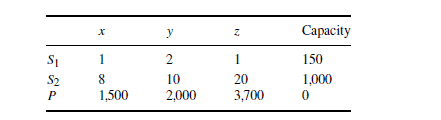
A farmer has 150 acres available to split between three crops: asparagus, beans, and corn. Each bag of asparagus seed is sufficient to plant 1 acre and requires 8 pounds of fertilizer. Each bag of bean seeds is sufficient to seed 2 acres and requires 10 pounds of fertilizer. Each bag of corn seed will plant 1 acre and requires 20 pounds of fertilizer. She has a total of $1,000 \mathrm{lbs}$. fertilizer to use on her two crops. The profit from a bag of asparagus seeds is $\$ 1,500$, and the profit from a bag of bean seeds is $\$ 2,000$. How many bags of each should she plant in order to maximize profit?
Let $x$ be the number of bags of asparagus seed.
Let $y$ be the number of bags of bean seed.
Let $z$ be the number of bags of corn seed.
Maximize: $P=1,500 x+2,000 y+3,700 z$
subject to:
$$
\begin{aligned}
&x+2 y+z \leq 150 \text { (acres land) } \
&8 x+10 y+20 z \leq 1,000 \text { (lbs. fertilizer) } \
&x \geq 0, y \geq 0, z \geq 0
\end{aligned}
$$
Observe that this is a $2 \times 3$ problem in standard form. We begin by arranging all the information in this problem in a table or matrix. It is a modified version of the augmented coefficient matrix of the system of equations (if we replaced the inequalities by equations.) See the following table.

凸优化代考

在第 1 章中，我们考虑了以下优化问题：以 80 英尺长的栅栏形成周长，最大面积的矩形花园的尺寸是多少 $x\times y$？我们看到解是当 $x=y=20$ 英尺时，所以解是正方形。当然，这不是线性规划问题，因为面积是由非线性函数 $A=x y$ 给出的。

一些思考可能会让读者相信这个问题可以被表述为一个最小化问题：如果一个矩形花园有 400 平方英尺的面积，那么什么尺寸产生的围栏数量最少（即最小周长）？解又是 $x=y=20$ 英尺，所以解是正方形。尽管这两个问题的表达方式不同，但它们都表达了正方形在某种意义上是最有效的矩形的想法。在所有周长固定的长方形中，正方形的面积最大；或者，等价地，在一个固定面积的所有矩形中，正方形的周长最小。

此示例表明，可能有两种方法可以表示单个优化问题，即最大化或最小化，具体取决于您将问题的哪一部分视为约束以及您将哪一部分视为目标函数。当优化问题是线性规划问题时，我们可以使这个想法非常精确。给定一个线性规划问题（我们称之为原始问题），还有另一个线性规划问题

最大化问题，对偶是最小化问题，当原始问题是最小化问题时，对偶是最大化问题。这些问题密切相关，从某种意义上说，它们可以看作是看待同一个问题的两种方式，并且具有“相同”的解决方案，就像在前面的例子中，两个关于矩形的问题的解决方案都是正方形。

对偶问题的概念具有重要的理论用途，它还提供了在进行某些计算时节省工作的工具。在本书中，我们不关心理论方面，将其留给编程和优化方面的更高级的文本。我们确实打算利用对偶的计算方面。在 4.5.1 节中，我们提出了一种寻找对偶问题的技术，而不用担心对偶问题的决策变量意味着什么。为了利用前面提到的计算捷径，这是一个人真正需要知道的关于对偶的全部内容。找到对偶的技术是机械的并且非常容易，但它没有暗示为什么这两个问题在概念上是联系在一起的。

该理论更有趣的方面是解释这两个问题如何相互关联。这在第 4.5.2 节中完成，我们在其中展示了如何解释对偶问题中的决策变量。打个比方，在第 4.5.1 节中，您将学习如何驾驶汽车，您无需了解任何关于内燃机的知识即可轻松做到这一点，而在第 4.5.2 节中，您将学习汽车的工作原理。在本书的后续章节中，只需要知道如何驾驶。
4.5.1 对偶的构建
我们使用标准形式的最大化问题作为原始问题来说明寻找对偶问题的技术。那么对偶总是标准形式的最小化问题。在 3.5 节中，我们讨论了以下问题（示例 3.12 的修改版本）：

一个农民有 150 英亩的土地可用于种植三种作物：芦笋、豆类和玉米。每袋芦笋种子足以种植 1 英亩，需要 8 磅肥料。每袋豆种子足以播种 2 英亩，需要 10 磅肥料。每袋玉米种子将种植 1 英亩，需要 20 磅肥料。她总共有 $1,000 \mathrm{lbs}$。肥料用于她的两种作物。一袋芦笋种子的利润是$\$ 1,500$，一袋豆子的利润是$\$ 2,000$。为了最大化利润，她每个应该种多少袋？
设 $x$ 为芦笋种子袋数。
设 $y$ 为豆种子袋数。
令 $z$ 为玉米种子袋数。
最大化：$P=1,500 x+2,000 y+3,700 z$
受制于：
$$
\开始{对齐}
&x+2 y+z \leq 150 \text { (英亩土地) } \
&8 x+10 y+20 z \leq 1,000 \text { (磅肥料) } \
&x \geq 0, y \geq 0, z \geq 0
\end{对齐}
$$
请注意，这是一个标准形式的 $2\times 3$ 问题。我们首先将这个问题中的所有信息安排在一个表格或矩阵中。它是方程组的增广系数矩阵的修改版本（如果我们用方程代替不等式）。见下表。