如果你也在 怎样代写有限元方法finite differences method 这个学科遇到相关的难题,请随时右上角联系我们的24/7代写客服。有限元方法finite differences method在数值分析中,是一类通过用有限差分逼近导数解决微分方程的数值技术。空间域和时间间隔(如果适用)都被离散化,或被分成有限的步骤,通过解决包含有限差分和附近点的数值的代数方程来逼近这些离散点的解的数值。
有限元方法finite differences method有限差分法将可能是非线性的常微分方程(ODE)或偏微分方程(PDE)转换成可以用矩阵代数技术解决的线性方程系统。现代计算机可以有效地进行这些线性代数计算,再加上其相对容易实现,使得FDM在现代数值分析中得到了广泛的应用。今天,FDM与有限元方法一样,是数值解决PDE的最常用方法之一。
有限元方法finite differences method作业代写,免费提交作业要求, 满意后付款,成绩80\%以下全额退款,安全省心无顾虑。专业硕 博写手团队,所有订单可靠准时,保证 100% 原创。 最高质量的有限元方法finite differences method作业代写,服务覆盖北美、欧洲、澳洲等 国家。 在代写价格方面,考虑到同学们的经济条件,在保障代写质量的前提下,我们为客户提供最合理的价格。 由于统计Statistics作业种类很多,同时其中的大部分作业在字数上都没有具体要求,因此有限元方法finite differences method作业代写的价格不固定。通常在经济学专家查看完作业要求之后会给出报价。作业难度和截止日期对价格也有很大的影响。
同学们在留学期间,都对各式各样的作业考试很是头疼,如果你无从下手,不如考虑my-assignmentexpert™!
my-assignmentexpert™提供最专业的一站式服务:Essay代写,Dissertation代写,Assignment代写,Paper代写,Proposal代写,Proposal代写,Literature Review代写,Online Course,Exam代考等等。my-assignmentexpert™专注为留学生提供Essay代写服务,拥有各个专业的博硕教师团队帮您代写,免费修改及辅导,保证成果完成的效率和质量。同时有多家检测平台帐号,包括Turnitin高级账户,检测论文不会留痕,写好后检测修改,放心可靠,经得起任何考验!
想知道您作业确定的价格吗? 免费下单以相关学科的专家能了解具体的要求之后在1-3个小时就提出价格。专家的 报价比上列的价格能便宜好几倍。
我们在数学Mathematics代写方面已经树立了自己的口碑, 保证靠谱, 高质且原创的数学Mathematics代写服务。我们的专家在微积分Calculus Assignment代写方面经验极为丰富,各种微积分Calculus Assignment相关的作业也就用不着 说。
数学代写|有限元方法作业代写finite differences method代考|Total Potential Energy
When $W_E$ involves only the work done by external forces that are independent of the deformation, we call it potential due to external loads and denote it by $V_E=W_E$ [see Eq. (2.3.3)]. The sum of the strain energy $U$ and the potential due to external forces $V_E$ is termed the total potential energy, and it is denoted by $\Pi=U+V_E\left(\sigma: \varepsilon=\sigma_{i j} \varepsilon_{i j}\right)$ :
$$
\Pi(\mathbf{u})=U+V_E=\frac{1}{2} \int_{\Omega} \sigma(\varepsilon): \varepsilon d \Omega-\left[\int_{\Omega} \mathbf{f} \cdot \mathbf{u} d \Omega+\oint_{\Gamma} \mathbf{t} \cdot \mathbf{u} d \Gamma\right]
$$
where $\Omega$ denotes the volume occupied by the body and $\Gamma$ is its total boundary.
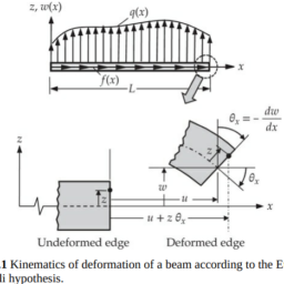
For example, the total potential energy expression for the Bernoulli-Euler beams (which include bars, i.e., members subjected to uniaxial forces as a special case) is
$$
\begin{aligned}
\Pi(u, w)= & \frac{1}{2} \int_0^L\left[E A\left(\frac{d u}{d x}\right)^2+E I\left(\frac{d^2 w}{d x^2}\right)^2\right] d x \
& -\left{\int_0^L[f(x) u(x)+q(x) w(x)] d x\right}
\end{aligned}
$$
where $f(x)$ is the distributed axial force along the line $z=0$ and $q(x)$ is the transverse distributed load at $z=h / 2$, both measured per unit length. The expression in Eq. (2.3.13) must be appended with any terms corresponding to the work done by external point forces and moments.
数学代写|有限元方法作业代写finite differences method代考|Strain Energy and Strain Energy Density
For deformable elastic bodies under isothermal conditions and infinitesimal deformations, the internal energy per unit volume, denoted by $U_0$ and termed strain energy density, consists of only stored elastic strain energy (for rigid bodies, $U_0=0$ ). An expression for strain energy density can be derived as follows.
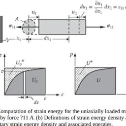
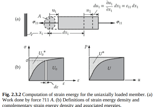
First, we consider axial deformation of a bar of area of cross section $A$. The free-body diagram of an element of length $d x_1$ of the bar is shown in Fig. 2.3.2(a). Note that the element is in static equilibrium, and we wish to determine the work done by the internal force associated with stress $\sigma_{11}^f$, where the superscript $f$ indicates that it is the final value of the quantity. Suppose that the element is deformed slowly so that axial strain varies from 0 to its final value $\varepsilon_{11}^f$. At any instant during the strain variation from $\varepsilon 11$ to $\varepsilon_{11}$ $+d \varepsilon_{11}$, we assume that $\sigma_{11}$ (due to $\varepsilon_{11}$ ) is kept constant so that equilibrium is maintained. Then the work done by the force $A \sigma_{11}$ in moving through the displacement $d \varepsilon_{11} d x_1$ is
$$
A \sigma_{11} d \varepsilon_{11} d x_1=\sigma_{11} d \varepsilon_{11}\left(A d x_1\right) \equiv d U_0\left(A d x_1\right)
$$
where $d U_0$ denotes the work done per unit volume in the element.
Referring to the stress-strain diagram in Fig. 2.3.2(b), $d U_0$ represents the elemental area under the stress-strain curve. The elemental area in the complement (in the rectangle formed by $\varepsilon_{11}$ and $\sigma_{11}$ ) is given by $d U_0^*=\varepsilon_{11} d \sigma_{11}$ and it is called the complementary strain energy density of the bar of length $d x_1$. In the present study, we will not be dealing with the complementary strain energy. The total area under the curve, $U_0$, is obtained
by integrating from zero to the final value of the strain (during which the stress changes according to its relation to the strain):
$$
U_0=\int_0^{\varepsilon_{11}} \sigma_{11} d \varepsilon_{11}
$$
where the superscript $f$ is omitted as the expression holds for any value of $\varepsilon$.
The internal work done (or strain energy stored) by $A \sigma_{11}$ over the whole element of length $d x$ during the entire deformation is
$$
d U=\int_0^{\varepsilon_{11}} \sigma_{11} d \varepsilon_{11}\left(A d x_1\right)=U_0\left(A d x_1\right)
$$
The total energy stored in the entire bar is obtained by integrating over the length of the bar:
$$
U=\int_0^L A U_0 d x_1
$$
This is the internal energy stored in the body due to deformation of the bar and it is called the strain energy. We note that no stress-strain relation is used, except that the stress-strain diagrams shown in Fig. 2.3.2(b) implies that it can be nonlinear. When the stress-strain relation is linear, say $\sigma_{11}=$ $E \varepsilon_{11}$, we have $U_0=(1 / 2) E \varepsilon_{11}^2=(1 / 2) \sigma_{11} \varepsilon_{11}$.
有限元方法代写
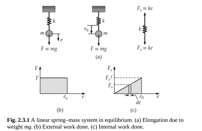
数学代写|有限元方法作业代写finite differences method代考|Work and Energy
由力(或力矩)所做的功定义为力(或力矩)与力(力矩)方向上的位移(或旋转)的乘积。因此,如果$\mathbf{F}$是力矢量$\mathbf{u}$是位移矢量,每个矢量都有自己的大小和方向,那么标量积(或点积)$\mathbf{F} \cdot \mathbf{u}$给出所做的功。所做的功是一个标量,单位是$\mathrm{N}-\mathrm{m}$(牛顿米)。当力和位移是位置$\mathbf{x}$在一个域$\Omega$中的函数时,则在该域上的积的积分给出所做的功:
$$
W=\int_{\Omega} \mathbf{F}(\mathbf{x}) \cdot \mathbf{u}(\mathbf{x}) d \Omega
$$
其中$d \Omega$表示物体的体积单元。如果$\mathbf{F}$也是$\mathbf{u}$的函数,则
$$
W=\int_{\Omega}\left(\int_0^{\mathbf{u}} \mathbf{F}(\mathbf{x}) \cdot d \mathbf{u}(\mathbf{x})\right) d \Omega
$$
为了进一步理解与位移无关的力和与位移有关的力所做的功之间的区别,考虑一个静力平衡的弹簧-质量系统[见图2.3.1(a)]。假设将质量$m$缓慢放置(为了消除动态影响)在线性弹性弹簧的末端(即弹簧中的力与弹簧中的位移成线性比例)。在固定大小的外力$F_0$的作用下,弹簧将拉长一个量$e_0$,从其未变形状态开始测量。在这种情况下,力$F_0$是由于重力,它等于$F_0=m g$。显然,$F_0$独立于春季的扩展$e_0$,并且$F_0$在扩展$e$从0到其最终值$e_0$的过程中没有变化[见图2.3.1(b)]。$F_0$通过$d e$所做的功是$F_0 d e$。那么$F_0$所做的(外部)总功为
$$
W_E=\int_0^{e_0} F_0 d e=F_0 e_0
$$
接下来考虑弹簧$F_s$中的力。弹簧中的力与弹簧中的位移成正比。因此,$F_s$的值从$e=0$时的0到$e=e_0$时的最终值$F_s^f$[见图2.3.1(c)]。$F_s$通过de所做的功是$F_s d e$。$F_s$完成的(内部)总功是
$$
W_I=\int_0^{e_0} F_s(e) d e
$$
数学代写|有限元方法作业代写finite differences method代考|Strain Energy and Strain Energy Density
对于等温条件和无穷小变形下的可变形弹性体,单位体积的内能,用$U_0$表示,称为应变能密度,仅由存储的弹性应变能组成(对于刚体,$U_0=0$)。应变能密度的表达式可推导为:
首先,我们考虑一根截面面积为$A$的杆的轴向变形。杆长为$d x_1$的单元的自由体图如图2.3.2(a)所示。注意,该元素处于静力平衡状态,我们希望确定与应力$\sigma_{11}^f$相关的内力所做的功,其中上标$f$表示它是该量的最终值。假设单元缓慢变形,轴向应变从0变化到最终值$\varepsilon_{11}^f$。在从$\varepsilon 11$到$\varepsilon_{11}$$+d \varepsilon_{11}$的应变变化过程中的任何时刻,我们假设$\sigma_{11}$(由于$\varepsilon_{11}$)保持不变,以保持平衡。那么力$A \sigma_{11}$通过位移$d \varepsilon_{11} d x_1$所做的功是
$$
A \sigma_{11} d \varepsilon_{11} d x_1=\sigma_{11} d \varepsilon_{11}\left(A d x_1\right) \equiv d U_0\left(A d x_1\right)
$$
其中$d U_0$表示单元中单位体积所做的功。
参考图2.3.2(b)的应力-应变图,$d U_0$表示应力-应变曲线下的元素面积。补片(由$\varepsilon_{11}$和$\sigma_{11}$组成的矩形)中的元素面积由$d U_0^*=\varepsilon_{11} d \sigma_{11}$给出,称为长度为$d x_1$的杆的补片应变能密度。在本研究中,我们将不处理互补应变能。曲线下的总面积为$U_0$
从0到应变的最终值(期间应力根据其与应变的关系变化)积分:
$$
U_0=\int_0^{\varepsilon_{11}} \sigma_{11} d \varepsilon_{11}
$$
其中省略上标$f$,因为表达式适用于$\varepsilon$的任何值。
在整个变形过程中,$A \sigma_{11}$在长度为$d x$的整个单元上所做的内功(或存储的应变能)为
$$
d U=\int_0^{\varepsilon_{11}} \sigma_{11} d \varepsilon_{11}\left(A d x_1\right)=U_0\left(A d x_1\right)
$$
储存在整个棒材中的总能量可通过对棒材长度积分得到:
$$
U=\int_0^L A U_0 d x_1
$$
这是由于杆的变形而储存在体内的内部能量,称为应变能。我们注意到没有使用应力-应变关系,除了图2.3.2(b)所示的应力-应变图表明它可能是非线性的。当应力应变关系是线性的,比如$\sigma_{11}=$$E \varepsilon_{11}$,我们有$U_0=(1 / 2) E \varepsilon_{11}^2=(1 / 2) \sigma_{11} \varepsilon_{11}$。

数学代写|有限元方法作业代写finite differences method代考 请认准UprivateTA™. UprivateTA™为您的留学生涯保驾护航。