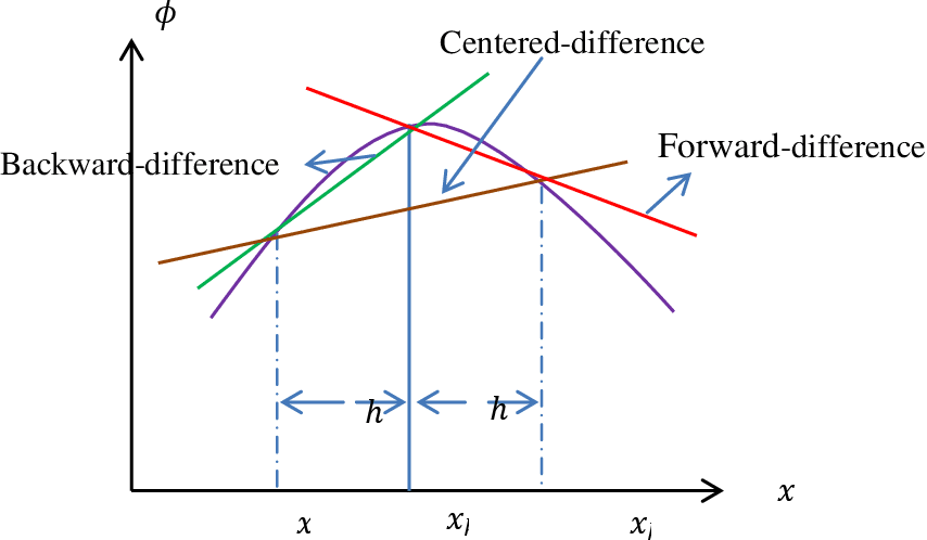
如果你也在 怎样代写有限元方法finite differences method 这个学科遇到相关的难题,请随时右上角联系我们的24/7代写客服。有限元方法finite differences method在数值分析中,是一类通过用有限差分逼近导数解决微分方程的数值技术。空间域和时间间隔(如果适用)都被离散化,或被分成有限的步骤,通过解决包含有限差分和附近点的数值的代数方程来逼近这些离散点的解的数值。
有限元方法finite differences method有限差分法将可能是非线性的常微分方程(ODE)或偏微分方程(PDE)转换成可以用矩阵代数技术解决的线性方程系统。现代计算机可以有效地进行这些线性代数计算,再加上其相对容易实现,使得FDM在现代数值分析中得到了广泛的应用。今天,FDM与有限元方法一样,是数值解决PDE的最常用方法之一。
有限元方法finite differences method作业代写,免费提交作业要求, 满意后付款,成绩80\%以下全额退款,安全省心无顾虑。专业硕 博写手团队,所有订单可靠准时,保证 100% 原创。 最高质量的有限元方法finite differences method作业代写,服务覆盖北美、欧洲、澳洲等 国家。 在代写价格方面,考虑到同学们的经济条件,在保障代写质量的前提下,我们为客户提供最合理的价格。 由于统计Statistics作业种类很多,同时其中的大部分作业在字数上都没有具体要求,因此有限元方法finite differences method作业代写的价格不固定。通常在经济学专家查看完作业要求之后会给出报价。作业难度和截止日期对价格也有很大的影响。
同学们在留学期间,都对各式各样的作业考试很是头疼,如果你无从下手,不如考虑my-assignmentexpert™!
my-assignmentexpert™提供最专业的一站式服务:Essay代写,Dissertation代写,Assignment代写,Paper代写,Proposal代写,Proposal代写,Literature Review代写,Online Course,Exam代考等等。my-assignmentexpert™专注为留学生提供Essay代写服务,拥有各个专业的博硕教师团队帮您代写,免费修改及辅导,保证成果完成的效率和质量。同时有多家检测平台帐号,包括Turnitin高级账户,检测论文不会留痕,写好后检测修改,放心可靠,经得起任何考验!
想知道您作业确定的价格吗? 免费下单以相关学科的专家能了解具体的要求之后在1-3个小时就提出价格。专家的 报价比上列的价格能便宜好几倍。
我们在数学Mathematics代写方面已经树立了自己的口碑, 保证靠谱, 高质且原创的数学Mathematics代写服务。我们的专家在微积分Calculus Assignment代写方面经验极为丰富,各种微积分Calculus Assignment相关的作业也就用不着 说。
数学代写|有限元方法作业代写finite differences method代考|The Basic Features of the Finite Element Method
The finite element method differs from the finite difference method in a fundamental way. The finite element method is a technique in which a dependent unknown is approximated as a linear combination of unknown parameters and known functions, whereas in the finite difference method the derivatives of the unknown are represented in terms of the values of the unknown. Thus, the finite difference method has no formal functional representation of the unknown itself; consequently, there are no evaluations of functions or their integrals, which can be considered as a positive aspect. However, there are associated drawbacks in imposing gradient boundary conditions and post-computation of gradients of the unknown. Further, the finite difference method only provides a means to compute solutions to problems described by differential equations but does not include the idea of minimizing the error in the approximation.
In a nutshell, the finite element method can be described as one that has the following three basic features:
Division of whole domain into subdomains, called finite elements, that enable a systematic derivation of the approximation functions as well as representation of complex domains.
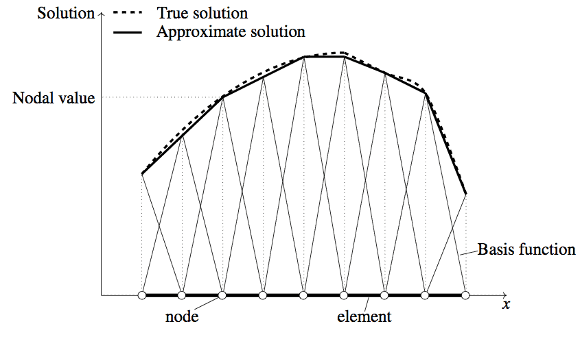
Discretization of the mathematical model of the problem (i.e., derivation of algebraic relations from governing equations) in terms of the values of the unknowns at selective points, called nodes, over each finite element. This step requires the use of an approximation method in which an unknown is represented as a linear combination of values of the unknown (and possibly its derivatives) at the nodes and suitable approximation functions, as discussed in Chapter 2. The element geometry and the position of the nodes in the element allow a systematic derivation of the approximation functions for each element. The approximation functions are often algebraic polynomials that are derived using interpolation theory. However, approximation functions need not be polynomials.
Assembly of the element equations to obtain a numerical analog of the mathematical model of the total problem being analyzed.
数学代写|有限元方法作业代写finite differences method代考|Discretization of a System
Most engineered systems are usually assemblages of subsystems. The smallest part that serves as the “building block” for the system or its subsystems and whose “cause and effect” relationships, the meaning of which will be made clear in the sequel, can be uniquely described mathematically is called an element. If a system has several subsystems that are different from each other in terms of their geometry and behavior, then each such subsystem is an assemblage of a unique type of element. Thus, a system may be assemblage of different types of elements (i.e., parts that have different physical behavior). An automobile is an assemblage of, for example, frame, doors, engine, and so on. Each of them may be characterized in terms of their load-deflection behavior as frame elements, shell elements, or threedimensional solid elements (see Fig. 1.4.8 for an example).
The phrase “discretization” in finite element analysis refers to representation of various parts of the system by a set of appropriate types of elements (e.g., frame element, shell element, or solid element). In general, such a representation is called a finite element mesh. In this introductory chapter, we will consider systems whose “cause and effect” can be described by only one type of element. Once we get comfortable, we can discuss multiple types of elements in a given system. In the following discussion, the word “domain” refers to the collection of material points of a continuous system whose physical behavior is of interest.
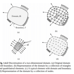
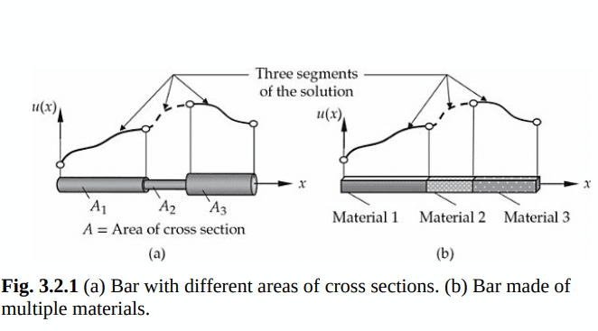
In the finite element method, the domain $\Omega$ of the problem is divided into a set of subdomains, called finite elements. The reason for dividing a domain into a set of subdomains is twofold. First, domains of most systems, by design, are a composite of geometrically and/or materially different parts, as shown in Fig. 3.2.1, and the solution on these subdomains is represented by different functions that are continuous at the interfaces of these subdomains. Therefore, it is appropriate to seek an approximation of the solution over each subdomain. Second, approximation of the solution over each element of the mesh is simpler than its approximation over the entire domain.
有限元方法代写
数学代写|有限元方法作业代写finite differences method代考|The Basic Features of the Finite Element Method
法是一种将依赖的未知近似为未知参数和已知函数的线性组合的技术,而在有限差分法中,未知的导数是用未知的值表示的。因此,有限差分法没有对未知本身的形式泛函表示;因此,没有对函数或其积分的评估,这可以被认为是一个积极的方面。然而,在施加梯度边界条件和未知梯度的后计算方面存在相关的缺陷。此外,有限差分法只提供了一种计算微分方程所描述问题的解的方法,而不包括在近似中使误差最小化的思想。
简而言之,有限元方法可以被描述为具有以下三个基本特征的方法:
将整个域划分为子域,称为有限元,从而可以系统地推导近似函数以及表示复杂域。
问题的数学模型的离散化(即,从控制方程中推导代数关系),根据每个有限单元上的选择点(称为节点)的未知量的值。这一步需要使用一种近似方法,在这种方法中,未知数被表示为节点处的未知数(可能还有它的导数)值和合适的近似函数的线性组合,如第2章所讨论的那样。元素的几何形状和节点在元素中的位置允许系统地推导每个元素的近似函数。逼近函数通常是利用插值理论推导出来的代数多项式。然而,近似函数不一定是多项式。
对单元方程进行装配,得到一个数值模拟的被分析总问题的数学模型。
数学代写|有限元方法作业代写finite differences method代考|Discretization of a System
大多数工程系统通常是子系统的组合。作为系统或子系统的“构建块”的最小部分,其“因果”关系(其含义将在后续文章中明确)可以用数学方法唯一地描述,称为元素。如果一个系统有几个子系统,它们在几何形状和行为方面彼此不同,那么每个这样的子系统都是一个独特类型元素的组合。因此,一个系统可能是不同类型的元素(即,具有不同物理行为的部件)的组合。汽车是诸如车架、车门、发动机等的组合。它们中的每一种都可以根据它们的载荷-挠度行为来表征为框架单元、壳单元或三维实体单元(示例见图1.4.8)。
有限元分析中的“离散化”是指用一组适当类型的单元(如框架单元、壳单元或实体单元)来表示系统的各个部分。一般来说,这样的表示称为有限元网格。在本导论章中,我们将考虑那些“因果关系”只能用一种元素来描述的系统。一旦我们适应了,我们就可以讨论给定系统中多种类型的元素。在接下来的讨论中,“域”一词指的是对其物理行为感兴趣的连续系统的物质点的集合。
在有限元法中,将问题的域$\Omega$划分为一组子域,称为有限元。将一个域划分为一组子域的原因有两个。首先,大多数系统的域被设计为几何和/或材料上不同部分的组合,如图3.2.1所示,并且这些子域上的解由在这些子域的接口处连续的不同函数表示。因此,在每个子域上寻求近似解是合适的。其次,在网格的每个元素上逼近解比在整个域上逼近解更简单。

数学代写|有限元方法作业代写finite differences method代考 请认准UprivateTA™. UprivateTA™为您的留学生涯保驾护航。