如果你也在 怎样代写有限元方法finite differences method 这个学科遇到相关的难题,请随时右上角联系我们的24/7代写客服。有限元方法finite differences method在数值分析中,是一类通过用有限差分逼近导数解决微分方程的数值技术。空间域和时间间隔(如果适用)都被离散化,或被分成有限的步骤,通过解决包含有限差分和附近点的数值的代数方程来逼近这些离散点的解的数值。
有限元方法finite differences method有限差分法将可能是非线性的常微分方程(ODE)或偏微分方程(PDE)转换成可以用矩阵代数技术解决的线性方程系统。现代计算机可以有效地进行这些线性代数计算,再加上其相对容易实现,使得FDM在现代数值分析中得到了广泛的应用。今天,FDM与有限元方法一样,是数值解决PDE的最常用方法之一。
有限元方法finite differences method作业代写,免费提交作业要求, 满意后付款,成绩80\%以下全额退款,安全省心无顾虑。专业硕 博写手团队,所有订单可靠准时,保证 100% 原创。 最高质量的有限元方法finite differences method作业代写,服务覆盖北美、欧洲、澳洲等 国家。 在代写价格方面,考虑到同学们的经济条件,在保障代写质量的前提下,我们为客户提供最合理的价格。 由于统计Statistics作业种类很多,同时其中的大部分作业在字数上都没有具体要求,因此有限元方法finite differences method作业代写的价格不固定。通常在经济学专家查看完作业要求之后会给出报价。作业难度和截止日期对价格也有很大的影响。
同学们在留学期间,都对各式各样的作业考试很是头疼,如果你无从下手,不如考虑my-assignmentexpert™!
my-assignmentexpert™提供最专业的一站式服务:Essay代写,Dissertation代写,Assignment代写,Paper代写,Proposal代写,Proposal代写,Literature Review代写,Online Course,Exam代考等等。my-assignmentexpert™专注为留学生提供Essay代写服务,拥有各个专业的博硕教师团队帮您代写,免费修改及辅导,保证成果完成的效率和质量。同时有多家检测平台帐号,包括Turnitin高级账户,检测论文不会留痕,写好后检测修改,放心可靠,经得起任何考验!
想知道您作业确定的价格吗? 免费下单以相关学科的专家能了解具体的要求之后在1-3个小时就提出价格。专家的 报价比上列的价格能便宜好几倍。
我们在数学Mathematics代写方面已经树立了自己的口碑, 保证靠谱, 高质且原创的数学Mathematics代写服务。我们的专家在微积分Calculus Assignment代写方面经验极为丰富,各种微积分Calculus Assignment相关的作业也就用不着 说。
数学代写|有限元方法作业代写finite differences method代考|Derivation of Element Equations: The Finite Element Model
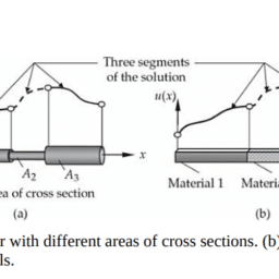
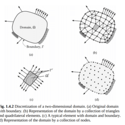
The domain and its subdivision into a collection of finite elements are shown in Fig. 3.4.2(a) and (b), respectively. A typical element, $\Omega^e=\left(x_a^e, x_b^e\right)$, is located between points A and B with coordinates $x=x_a^e$ and $x=x_b^e$ and its length is $h_e=x_b^e-x_a^e$. The collection of finite elements in a domain is called the finite element mesh of the domain. To obtain the Ritz equations for the nodal values of $u(x)$, we focus on solving Eq. (3.4.1) subject to the boundary conditions $u\left(x_a^e\right)=u_a^e$ and $u\left(x_b^e\right)=u_b^e$ using the Ritz method. The main difference here is that we apply a variational method over a finite element $\Omega^e$ as opposed to the total domain $\Omega$. This step results in the finite element model, $\mathbf{K}^e \mathbf{u}^e=\mathbf{F}^e$.
The derivation of finite element equations, that is, algebraic relations among the unknown parameters of the finite element approximation, involves the following three steps:
Construct the weighted-residual or weak form of the differential equation.
Assume the form of the approximate solution over a typical finite element.
Derive the finite element equations by substituting the approximate solution into the weighted-residual or weak form.
A typical element $\Omega^e=\left(x_a^e, x_b^e\right)$ is isolated from the mesh [see Fig. 3.4.3(a) and (b)]. We seek an approximate solution to the governing differential equation over the element. In principle, any method of solution that allows the derivation of necessary algebraic relations among the duality pairs at all nodes of the element can be used. In this book we develop the algebraic equations using the Ritz (i.e., the weak-form Galerkin) method.
数学代写|有限元方法作业代写finite differences method代考|Weak-form development
The weak-form development was discussed in detail in Sections 2.4.4-2.4.6. Here we review the three steps in the derivation of the weak form associated with the model differential equation over a typical element of the mesh. We begin with the polynomial approximation of the solution within a typical finite element $\Omega^e$ to be of the form:
$$
u_h^e(x)=\sum_{j=1}^n u_j^e \psi_j^e(x)
$$
where $u_j^e$ are the values of the solution $u(x)$ at the nodes of the finite element $\Omega^e$, and $\psi_j^e(x)$ are the approximation functions over the element. The superscript $e$ refers to element $\Omega^e$ while the subscript $h$ on the approximate solution $u_h^e$ refers to a mesh parameter (such as the length of the element). The particular form in Eq. (3.4.3) will be derived in the next section. Note that the approximation in Eq. (3.4.3) differs from the one used in the Ritz method in that $c_j \varphi_j(x)$ is now replaced with $u_j^e \psi_j^e(x)$, and $u_j^e$ plays the role of undetermined parameters and $\psi_j^e$ the role of approximation functions over an element $\Omega^e$. As we shall see later, writing the approximation in terms of the nodal values of the solution is necessitated by the fact that the continuity of $u(x)$ between elements can be readily imposed by equating the nodal values from all elements connected at the node. In addition, when the final algebraic equations are solved we obtain the nodal values $u_j^e$ directly as opposed to parameters $c_j$, which often do not have any physical meaning.
Since the actual solution $u$ is replaced by its approximation $u_h^e$ over an element $\Omega^e$, the left side of Eq. (3.4.1) will not be equal to zero in $\Omega^e$. The error in the approximation of the differential equation is denoted by $R^e$ and it is called the residual:
$$
R^e\left(x, u_h^e\right) \equiv-\frac{d}{d x}\left(a_e \frac{d u_h^e}{d x}\right)+c_e u_h^e-f_e \neq 0 \quad \text { for } \quad x_a^e<x<x_b^e
$$
where $a_e, c_e$, and $f_e$ are element-wise continuous functions. Since $u_h^e(x)$ is expressed as a linear combination of the unknown coefficients $u_j^e$, we wish to determine them by requiring the residual $R^e$ to be zero in an integral sense. The necessary and sufficient number $(n)$ of algebraic relations among the $u_j^e$ can be obtained only by forcing the integral of the weighted-residual to zero (the first step of the weak-form development):
$$
0=\int_{x^e}^{x_b^e} w_i^e(x) R^e\left(x, u_h^e\right) d x=\int_{x^e}^{x_b^e} w_i^e\left[-\frac{d}{d x}\left(a_e \frac{d u_h^e}{d x}\right)+c_e u_h^e-f_e\right] d x
$$
有限元方法代写
数学代写|有限元方法作业代写finite differences method代考|Derivation of Element Equations: The Finite Element Model
区域及其细分为有限元集合分别如图3.4.2(a)和(b)所示。典型的元素$\Omega^e=\left(x_a^e, x_b^e\right)$位于点A和点B之间,坐标分别为$x=x_a^e$和$x=x_b^e$,其长度为$h_e=x_b^e-x_a^e$。一个域内的有限元集合称为该域的有限元网格。为了得到$u(x)$节点值的Ritz方程,我们重点使用Ritz方法求解边界条件$u\left(x_a^e\right)=u_a^e$和$u\left(x_b^e\right)=u_b^e$下的Eq.(3.4.1)。这里的主要区别在于,我们在有限元$\Omega^e$上应用变分方法,而不是在总域$\Omega$上。这一步得到有限元模型$\mathbf{K}^e \mathbf{u}^e=\mathbf{F}^e$ .
有限元方程的推导,即有限元逼近的未知参数之间的代数关系,包括以下三个步骤:
构造微分方程的加权残差或弱形式。
假设典型有限元近似解的形式。
通过将近似解代入加权残差或弱形式来推导有限元方程。
从网格中分离出一个典型单元$\Omega^e=\left(x_a^e, x_b^e\right)$[见图3.4.3(A)和(b)]。我们求对该元素的控制微分方程的近似解。原则上,任何允许在元素的所有节点的对偶对之间推导必要的代数关系的解方法都可以使用。在这本书中,我们使用Ritz(即弱形式Galerkin)方法来发展代数方程。
数学代写|有限元方法作业代写finite differences method代考|Weak-form development
弱形式开发已在第2.4.4-2.4.6节中详细讨论。在这里,我们回顾了与典型网格单元上的模型微分方程相关的弱形式推导的三个步骤。我们从典型有限元$\Omega^e$中解的多项式近似开始,其形式为:
$$
u_h^e(x)=\sum_{j=1}^n u_j^e \psi_j^e(x)
$$
其中$u_j^e$是有限元$\Omega^e$节点处的解$u(x)$的值,$\psi_j^e(x)$是单元上的近似函数。上标$e$指的是元素$\Omega^e$,而近似解$u_h^e$上的下标$h$指的是网格参数(如元素的长度)。方程(3.4.3)中的具体形式将在下一节推导。请注意,Eq.(3.4.3)中的近似与Ritz方法中使用的近似不同,因为$c_j \varphi_j(x)$现在被$u_j^e \psi_j^e(x)$取代,$u_j^e$扮演待定参数的角色,$\psi_j^e$扮演元素$\Omega^e$上的近似函数的角色。正如我们将在后面看到的,用解的节点值来写近似是必要的,因为通过在节点上连接的所有元素的节点值相等,可以很容易地实现元素之间$u(x)$的连续性。此外,在求解最终代数方程时,我们直接获得节点值$u_j^e$,而不是参数$c_j$,后者通常没有任何物理意义。
由于实际解$u$被其在元素$\Omega^e$上的近似值$u_h^e$所取代,因此公式(3.4.1)的左侧在$\Omega^e$中不等于零。微分方程的近似误差用$R^e$表示,它被称为残差:
$$
R^e\left(x, u_h^e\right) \equiv-\frac{d}{d x}\left(a_e \frac{d u_h^e}{d x}\right)+c_e u_h^e-f_e \neq 0 \quad \text { for } \quad x_a^e<x<x_b^e
$$
其中$a_e, c_e$和$f_e$是单元连续函数。由于$u_h^e(x)$表示为未知系数$u_j^e$的线性组合,我们希望通过要求残差$R^e$在积分意义上为零来确定它们。只有将加权残差的积分强制为零(弱形式展开的第一步),才能得到$u_j^e$之间代数关系的充分必要数$(n)$:
$$
0=\int_{x^e}^{x_b^e} w_i^e(x) R^e\left(x, u_h^e\right) d x=\int_{x^e}^{x_b^e} w_i^e\left[-\frac{d}{d x}\left(a_e \frac{d u_h^e}{d x}\right)+c_e u_h^e-f_e\right] d x
$$

数学代写|有限元方法作业代写finite differences method代考 请认准UprivateTA™. UprivateTA™为您的留学生涯保驾护航。