如果你也在 怎样代写有限元方法finite differences method 这个学科遇到相关的难题,请随时右上角联系我们的24/7代写客服。有限元方法finite differences method在数值分析中,是一类通过用有限差分逼近导数解决微分方程的数值技术。空间域和时间间隔(如果适用)都被离散化,或被分成有限的步骤,通过解决包含有限差分和附近点的数值的代数方程来逼近这些离散点的解的数值。
有限元方法finite differences method有限差分法将可能是非线性的常微分方程(ODE)或偏微分方程(PDE)转换成可以用矩阵代数技术解决的线性方程系统。现代计算机可以有效地进行这些线性代数计算,再加上其相对容易实现,使得FDM在现代数值分析中得到了广泛的应用。今天,FDM与有限元方法一样,是数值解决PDE的最常用方法之一。
有限元方法finite differences method作业代写,免费提交作业要求, 满意后付款,成绩80\%以下全额退款,安全省心无顾虑。专业硕 博写手团队,所有订单可靠准时,保证 100% 原创。 最高质量的有限元方法finite differences method作业代写,服务覆盖北美、欧洲、澳洲等 国家。 在代写价格方面,考虑到同学们的经济条件,在保障代写质量的前提下,我们为客户提供最合理的价格。 由于统计Statistics作业种类很多,同时其中的大部分作业在字数上都没有具体要求,因此有限元方法finite differences method作业代写的价格不固定。通常在经济学专家查看完作业要求之后会给出报价。作业难度和截止日期对价格也有很大的影响。
同学们在留学期间,都对各式各样的作业考试很是头疼,如果你无从下手,不如考虑my-assignmentexpert™!
my-assignmentexpert™提供最专业的一站式服务:Essay代写,Dissertation代写,Assignment代写,Paper代写,Proposal代写,Proposal代写,Literature Review代写,Online Course,Exam代考等等。my-assignmentexpert™专注为留学生提供Essay代写服务,拥有各个专业的博硕教师团队帮您代写,免费修改及辅导,保证成果完成的效率和质量。同时有多家检测平台帐号,包括Turnitin高级账户,检测论文不会留痕,写好后检测修改,放心可靠,经得起任何考验!
想知道您作业确定的价格吗? 免费下单以相关学科的专家能了解具体的要求之后在1-3个小时就提出价格。专家的 报价比上列的价格能便宜好几倍。
我们在数学Mathematics代写方面已经树立了自己的口碑, 保证靠谱, 高质且原创的数学Mathematics代写服务。我们的专家在微积分Calculus Assignment代写方面经验极为丰富,各种微积分Calculus Assignment相关的作业也就用不着 说。
数学代写|有限元方法作业代写finite differences method代考|Postprocessing of the Solution
Once the boundary conditions are imposed, the resulting (condensed) equations are solved for the unknown generalized nodal displacements. The generalized forces can be computed using the condensed equations for the unknown reactions. However, this is seldom the case in practice, because the assembled equations are modified to solve for the unknown primary variables (i.e., generalized displacements). Therefore, the generalized forces are
computed using the known displacement field.
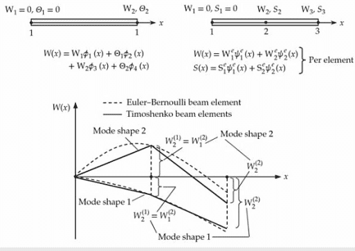
The solution $w_h^e$ and its slope $\theta_x^e$ in each element $\Omega^e=\left(x_a^e, x_a^e\right)$ are given by
$$
w_h^e(\bar{x})=\sum_{j=1}^4 \Delta_j^e \phi_j^e(\bar{x}), \quad \theta_x^e(x)=-\frac{d w_h^e}{d x}=-\sum_{j=1}^4 \Delta_j^e \frac{d \phi_j^e}{d \bar{x}}, 0 \leq \bar{x} \leq h_e
$$
The bending moment $M$ and shear force $V$ at any point in the element $\Omega^e$ of the beam can be post-computed from the finite element solution $w_h^e(\bar{x}), 0 \leq \bar{x} \leq h_e$, using
$$
\begin{aligned}
& M_h^e(\bar{x})=-E_e I_e \frac{d^2 w_h^e}{d \bar{x}^2} \approx-E_e I_e \sum_{j=1}^4 \Delta_j^e \frac{d^2 \phi_j^e}{d \bar{x}^2} \
& V_h^e(\bar{x})=-\frac{d}{d \bar{x}}\left(E_e I_e \frac{d^2 w_h^e}{d \bar{x}^2}\right) \approx-\frac{d}{d \bar{x}}\left(E_e I_e \sum_{j=1}^4 \Delta_j^e \frac{d^2 \phi_j^e}{d \bar{x}^2}\right)
\end{aligned}
$$
数学代写|有限元方法作业代写finite differences method代考|Beams with internal hinge
It is not uncommon to find beams with an internal hinge about which the beam is free to rotate. Thus, at the hinge there cannot be any moment and the rotation is not continuous at a hinge between two elements (i.e., two elements connected at a hinge will have two different rotations). The assembly of element equations becomes simple if we eliminate the rotation variable at a node with a hinge.
Consider a uniform beam element of length $h_e$ with a hinge at node 2 (but without elastic foundation, $k_f=0$ ), as shown in Fig. 5.2.17(a). The element equation is given by Eq. (5.2.25), with the stiffness matrix given in Eq. $(5.2 .26 a):$
$$
\frac{2 E_e I_e}{h_e^3}\left[\begin{array}{cccc}
6 & -3 h_e & -6 & -3 h_e \
-3 h_e & 2 h_e^2 & 3 h_e & h_e^2 \
-6 & 3 h_e & 6 & 3 h_e \
-3 h_e & h_e^2 & 3 h_e & 2 h_e^2
\end{array}\right]\left{\begin{array}{c}
w_1^e \
\theta_1^e \
w_2^e \
\theta_2^e
\end{array}\right}=\left{\begin{array}{l}
q_1^e \
q_2^e \
q_3^e \
q_4^e
\end{array}\right}+\left{\begin{array}{l}
Q_1^e \
Q_2^e \
Q_3^e \
Q_4^e
\end{array}\right}
$$
Since the moment at a hinge is zero, we have $Q_4^e=0$. This allows us to eliminate $\theta_2^e$ (rotation at node 2) using the procedure discussed in Eqs. $(3.4 .57)-(3.4 .61)$
Comparing Eq. (5.2.39) with Eq. (3.4.57), we have the following definitions:
$$
\begin{gathered}
\mathbf{K}^{11}=\frac{2 E_e I_e}{h_e^3}\left[\begin{array}{ccc}
6 & -3 h_e & -6 \
-3 h_e & 2 h_e^2 & 3 h_e \
-6 & 3 h_e & 6
\end{array}\right], \quad \mathbf{K}^{12}=\frac{2 E_e I_e}{h_e^3}\left{\begin{array}{c}
-3 h_e \
h_e^2 \
3 h_e
\end{array}\right}=\left(\mathbf{K}^{21}\right)^{\mathrm{T}} \
\mathbf{K}^{22}=\frac{4 E_e I_e}{h_e}, \quad \mathbf{U}^1=\left{\begin{array}{c}
w_1^e \
\theta_1^e \
w_2^2
\end{array}\right}, \quad \mathbf{U}^2=\theta_2^e, \quad \mathbf{F}^1=\left{\begin{array}{c}
q_1^e \
q_2^e \
q_3^e
\end{array}\right}+\left{\begin{array}{c}
Q_1^e \
Q_2^e \
Q_3^e
\end{array}\right}
\end{gathered}
$$
有限元方法代写
数学代写|有限元方法作业代写finite differences method代考|Postprocessing of the Solution
一旦施加边界条件,则求解未知广义节点位移的结果(浓缩)方程。广义力可以用未知反应的简化方程来计算。然而,在实践中很少出现这种情况,因为组合方程被修改以求解未知的主要变量(即广义位移)。因此,广义力
用已知位移场计算。
每个单元$\Omega^e=\left(x_a^e, x_a^e\right)$的解$w_h^e$及其斜率$\theta_x^e$由
$$
w_h^e(\bar{x})=\sum_{j=1}^4 \Delta_j^e \phi_j^e(\bar{x}), \quad \theta_x^e(x)=-\frac{d w_h^e}{d x}=-\sum_{j=1}^4 \Delta_j^e \frac{d \phi_j^e}{d \bar{x}}, 0 \leq \bar{x} \leq h_e
$$给出
梁的$\Omega^e$单元中任意点的弯矩$M$和剪力$V$可由有限元解$w_h^e(\bar{x}), 0 \leq \bar{x} \leq h_e$后算,使用
$$
\begin{aligned}
& M_h^e(\bar{x})=-E_e I_e \frac{d^2 w_h^e}{d \bar{x}^2} \approx-E_e I_e \sum_{j=1}^4 \Delta_j^e \frac{d^2 \phi_j^e}{d \bar{x}^2} \
& V_h^e(\bar{x})=-\frac{d}{d \bar{x}}\left(E_e I_e \frac{d^2 w_h^e}{d \bar{x}^2}\right) \approx-\frac{d}{d \bar{x}}\left(E_e I_e \sum_{j=1}^4 \Delta_j^e \frac{d^2 \phi_j^e}{d \bar{x}^2}\right)
\end{aligned}
$$
数学代写|有限元方法作业代写finite differences method代考|Beams with internal hinge
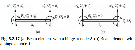
找到具有内部铰链的梁并不罕见,梁可以围绕其自由旋转。因此,在铰链处不可能有任何力矩,两个元件之间的铰链处的旋转是不连续的(即在铰链处连接的两个元件会有两次不同的旋转)。如果我们消除带有铰链的节点上的旋转变量,单元方程的装配就会变得简单。
考虑长度为$h_e$的均匀梁单元,节点2处有铰(但不含弹性基础$k_f=0$),如图5.2.17(a)所示。单元方程由式(5.2.25)给出,其中刚度矩阵为式$(5.2 .26 a):$
$$
\frac{2 E_e I_e}{h_e^3}\left[\begin{array}{cccc}
6 & -3 h_e & -6 & -3 h_e \
-3 h_e & 2 h_e^2 & 3 h_e & h_e^2 \
-6 & 3 h_e & 6 & 3 h_e \
-3 h_e & h_e^2 & 3 h_e & 2 h_e^2
\end{array}\right]\left{\begin{array}{c}
w_1^e \
\theta_1^e \
w_2^e \
\theta_2^e
\end{array}\right}=\left{\begin{array}{l}
q_1^e \
q_2^e \
q_3^e \
q_4^e
\end{array}\right}+\left{\begin{array}{l}
Q_1^e \
Q_2^e \
Q_3^e \
Q_4^e
\end{array}\right}
$$
由于铰处弯矩为零,我们得到$Q_4^e=0$。这允许我们使用公式中讨论的过程消除$\theta_2^e$(节点2的旋转)。$(3.4 .57)-(3.4 .61)$
将Eq.(5.2.39)与Eq.(3.4.57)进行比较,我们得到以下定义:
$$
\begin{gathered}
\mathbf{K}^{11}=\frac{2 E_e I_e}{h_e^3}\left[\begin{array}{ccc}
6 & -3 h_e & -6 \
-3 h_e & 2 h_e^2 & 3 h_e \
-6 & 3 h_e & 6
\end{array}\right], \quad \mathbf{K}^{12}=\frac{2 E_e I_e}{h_e^3}\left{\begin{array}{c}
-3 h_e \
h_e^2 \
3 h_e
\end{array}\right}=\left(\mathbf{K}^{21}\right)^{\mathrm{T}} \
\mathbf{K}^{22}=\frac{4 E_e I_e}{h_e}, \quad \mathbf{U}^1=\left{\begin{array}{c}
w_1^e \
\theta_1^e \
w_2^2
\end{array}\right}, \quad \mathbf{U}^2=\theta_2^e, \quad \mathbf{F}^1=\left{\begin{array}{c}
q_1^e \
q_2^e \
q_3^e
\end{array}\right}+\left{\begin{array}{c}
Q_1^e \
Q_2^e \
Q_3^e
\end{array}\right}
\end{gathered}
$$

数学代写|有限元方法作业代写finite differences method代考 请认准UprivateTA™. UprivateTA™为您的留学生涯保驾护航。