如果你也在 怎样代写有限元方法finite differences method 这个学科遇到相关的难题,请随时右上角联系我们的24/7代写客服。有限元方法finite differences method领域中所有的物理系统都可以用边界/初值问题来表示。在这本书中,我们主要集中在解决一维和二维线性弹性和传热问题。将这些解决方案技术扩展到三维分析是直接的,因此为了保持表示的清晰性并避免重复,这里不进行讨论。
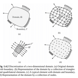
有限元方法finite differences method提供了一种系统的方法来推导简单子区域的近似函数,通过这些近似函数可以表示几何上复杂的区域。在有限元法中,近似函数是分段多项式(即只在子区域上定义的多项式,称为单元)。
有限元方法finite differences method作业代写,免费提交作业要求, 满意后付款,成绩80\%以下全额退款,安全省心无顾虑。专业硕 博写手团队,所有订单可靠准时,保证 100% 原创。 最高质量的有限元方法finite differences method作业代写,服务覆盖北美、欧洲、澳洲等 国家。 在代写价格方面,考虑到同学们的经济条件,在保障代写质量的前提下,我们为客户提供最合理的价格。 由于统计Statistics作业种类很多,同时其中的大部分作业在字数上都没有具体要求,因此有限元方法finite differences method作业代写的价格不固定。通常在经济学专家查看完作业要求之后会给出报价。作业难度和截止日期对价格也有很大的影响。
同学们在留学期间,都对各式各样的作业考试很是头疼,如果你无从下手,不如考虑my-assignmentexpert™!
my-assignmentexpert™提供最专业的一站式服务:Essay代写,Dissertation代写,Assignment代写,Paper代写,Proposal代写,Proposal代写,Literature Review代写,Online Course,Exam代考等等。my-assignmentexpert™专注为留学生提供Essay代写服务,拥有各个专业的博硕教师团队帮您代写,免费修改及辅导,保证成果完成的效率和质量。同时有多家检测平台帐号,包括Turnitin高级账户,检测论文不会留痕,写好后检测修改,放心可靠,经得起任何考验!
想知道您作业确定的价格吗? 免费下单以相关学科的专家能了解具体的要求之后在1-3个小时就提出价格。专家的 报价比上列的价格能便宜好几倍。
我们在数学Mathematics代写方面已经树立了自己的口碑, 保证靠谱, 高质且原创的数学Mathematics代写服务。我们的专家在微积分Calculus Assignment代写方面经验极为丰富,各种微积分Calculus Assignment相关的作业也就用不着 说。
数学代写|有限元方法作业代写finite differences method代考|Weak form of EBT
The weak form of the equation governing the EBT, Eq. (7.3.31), is given by
$$
\begin{aligned}
0= & \int_{x_a^e}^{x_b^e}\left(E I \frac{d^2 v}{d x^2} \frac{d^2 W}{d x^2}-N^0 \frac{d v}{d x} \frac{d W}{d x}\right) d x \
& -v\left(x_a^e\right) Q_1^e-\left(-\frac{d v}{d x}\right){x_a^e} Q_2^e-v\left(x_b^e\right) Q_3^e-\left(-\frac{d v}{d x}\right){x_b^e} Q_4^e
\end{aligned}
$$
where $v$ is the weight function and
$$
\begin{array}{ll}
Q_1^e=\left[\frac{d}{d x}\left(E I \frac{d^2 W}{d x^2}\right)+N^0 \frac{d W}{d x}\right]{x_a^e}, \quad Q_2^e=\left(E I \frac{d^2 W}{d x^2}\right){x_a^e} \
Q_3^e=\left[-\frac{d}{d x}\left(E I \frac{d^2 W}{d x^2}\right)-N^0 \frac{d W}{d x}\right]{x_b^e}, & Q_4^e=\left(-E I \frac{d^2 W}{d x^2}\right){x_b^e}
\end{array}
$$
Clearly, the duality pairs of the weak form are $(W, V)$ and $(-d W / d x, M)$. We note that for the buckling problem, the buckling load is a part of the shear forces $Q_1^e$ and $Q_3^e$ because it contributes to the reaction forces.
The finite element model is obtained by approximating $W(x)$ such that both $W$ and its derivative $(-d W / d x)$ are interpolated at the nodes of the element. As already discussed in Chapter 5 (see Section 5.2.4), the minimum degree of interpolation of $W$ is cubic:
$$
W(x) \approx \sum_{j=1}^4 \Delta_j^e \phi_j^e(x)
$$
where $\phi_j(x)$ are the Hermite cubic polynomials given in Eq. (5.2.20). Substituting Eq. (7.3.67) into the weak form (7.3.66a), we obtain the finite element model
$$
\mathbf{K}^e \Delta^e-N^0 \mathbf{G}^e \boldsymbol{\Delta}^e=\mathbf{Q}^e
$$
where $\boldsymbol{\Delta}^e$ and $\mathbf{Q}^e$ are the columns of generalized displacement and force degrees of freedom at the two ends of the Euler-Bernoulli beam element:
$$
\Delta^e=\left{\begin{array}{c}
W\left(x_a^e\right) \
\left(-\frac{d W}{d x}\right){x_a^e} \ W\left(x_b^e\right)^e \ \left(-\frac{d W}{d x}\right){x_k^e}
\end{array}\right}, \quad \mathbf{Q}^e=\left{\begin{array}{l}
Q_1^e \
Q_2^e \
Q_3^e \
Q_4^e
\end{array}\right}
$$
The coefficients of the stiffness matrix $\mathbf{K}^e$ and the stability matrix $\mathbf{G}^e$ are defined by
$$
K_{i j}^e=\int_{x_a}^{x_b} E I \frac{d^2 \phi_i^e}{d x^2} \frac{d^2 \phi_j^e}{d x^2} d x, \quad G_{i j}^e=\int_{x_a}^{x_b} \frac{d \phi_i^e}{d x} \frac{d \phi_j^e}{d x} d x
$$
where $\phi_i^e$ are the Hermite cubic interpolation functions. The explicit form of $\mathbf{K}^e$ is given by Eq. (5.2.26a) with $k_f^e=0$ for element-wise constant value of $E_e I_e$. The element equations for buckling of a beam-column according to the Euler-Bernoulli beam theory (for the case $k_f^e=0$ ) are
$$
\begin{gathered}
\left(\frac{2 E_e I_e}{h_e^3}\left[\begin{array}{cccc}
6 & -3 h_e & -6 & -3 h_e \
-3 h_e & 2 h_e^2 & 3 h_e & h_e^2 \
-6 & 3 h_e & 6 & 3 h_e \
-3 h_e & h_e^2 & 3 h_e & 2 h_e^2
\end{array}\right]\right. \
\left.-N^0 \frac{1}{30 h_e}\left[\begin{array}{cccc}
36 & -3 h_e & -36 & -3 h_e \
-3 h_e & 4 h_e^2 & 3 h_e & -h_e^2 \
-36 & 3 h_e & 36 & 3 h_e \
-3 h_e & -h_e^2 & 3 h_e & 4 h_e^2
\end{array}\right]\right)\left{\begin{array}{c}
\Delta_1^e \
\Delta_2^e \
\Delta_3^e \
\Delta_4^e
\end{array}\right}=\left{\begin{array}{l}
Q_1^e \
Q_2^e \
Q_3^e \
Q_4^e
\end{array}\right}
\end{gathered}
$$
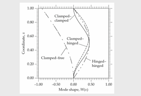
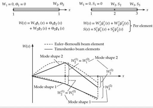
The mode shape in the element is given by Eq. (7.3.67).
数学代写|有限元方法作业代写finite differences method代考|Weak form
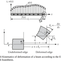
We begin with the development of the weak form of Eq. (7.4.3) over an element for any arbitrary time, followed by the derivation of the semidiscrete finite element model using the approximation of the form in Eq. (7.4.1b). Following the three-step procedure of constructing the weak form of a differential equation (all of the terms in the differential equation have already been considered previously), we obtain
$$
\begin{aligned}
0= & \int_{x_e^e}^{x_b^e}\left[a \frac{d w}{d x} \frac{\partial u}{\partial x}+b \frac{d^2 w}{d x^2} \frac{\partial^2 u}{\partial x^2}+c_3 \frac{d w}{d x} \frac{\partial^3 u}{\partial x \partial t^2}+w\left(c_0 u+c_1 \frac{\partial u}{\partial t}+c_2 \frac{\partial^2 u}{\partial t^2}-f\right)\right] d x \
& +\left[w\left(-a \frac{\partial u}{\partial x}+\frac{\partial}{\partial x}\left(b \frac{\partial^2 u}{\partial x^2}\right)-c_3 \frac{\partial^3 u}{\partial x \partial t^2}\right)+\frac{d w}{d x}\left(-b \frac{\partial^2 u}{\partial x^2}\right)\right]{x_a^e}^{x_b^e} \ = & \int{x_e^e}^{x_b^e}\left[a \frac{d w}{d x} \frac{\partial u}{\partial x}+b \frac{d^2 w}{d x^2} \frac{\partial^2 u}{\partial x^2}+c_3 \frac{d w}{d x} \frac{\partial^3 u}{\partial x \partial t^2}+w\left(c_0 u+c_1 \frac{\partial u}{\partial t}+c_2 \frac{\partial^2 u}{\partial t^2}-f\right)\right] d x \
& -Q_1^e w\left(x_a^e\right)-Q_3^e w\left(x_b^e\right)-\left.Q_2^e\left(-\frac{d w}{d x}\right)\right|{x_a^e}-\left.Q_4^e\left(-\frac{d w}{d x}\right)\right|{x_b^e}
\end{aligned}
$$
where $w(x)$ is the weight function and
$$
\begin{aligned}
& Q_1^e=\left[-a \frac{\partial u}{\partial x}+\frac{\partial}{\partial x}\left(b \frac{\partial^2 u}{\partial x^2}\right)-c_3 \frac{\partial^3 u}{\partial x \partial t^2}\right]{x_a^e}, \quad Q_2^c=\left[b \frac{\partial^2 u}{\partial x^2}\right]{x_a^e} \
& Q_3^e=-\left[-a \frac{\partial u}{\partial x}+\frac{\partial}{\partial x}\left(b \frac{\partial^2 u}{\partial x^2}\right)-c_3 \frac{\partial^3 u}{\partial x \partial t^2}\right]{x_b^e}, \quad Q_4^c=-\left[b \frac{\partial^2 u}{\partial x^2}\right]{x_b^e}
\end{aligned}
$$
We note that the primary variables are $u$ and $\partial u / \partial x$. Therefore, the finite element approximation of $u(x, t)$ is necessarily based on the Hermite cubic polynomials.
有限元方法代写
数学代写|有限元方法作业代写finite differences method代考|Weak form of EBT
控制EBT的方程的弱形式,方程(7.3.31),由
$$
\begin{aligned}
0= & \int_{x_a^e}^{x_b^e}\left(E I \frac{d^2 v}{d x^2} \frac{d^2 W}{d x^2}-N^0 \frac{d v}{d x} \frac{d W}{d x}\right) d x \
& -v\left(x_a^e\right) Q_1^e-\left(-\frac{d v}{d x}\right){x_a^e} Q_2^e-v\left(x_b^e\right) Q_3^e-\left(-\frac{d v}{d x}\right){x_b^e} Q_4^e
\end{aligned}
$$
$v$是权重函数
$$
\begin{array}{ll}
Q_1^e=\left[\frac{d}{d x}\left(E I \frac{d^2 W}{d x^2}\right)+N^0 \frac{d W}{d x}\right]{x_a^e}, \quad Q_2^e=\left(E I \frac{d^2 W}{d x^2}\right){x_a^e} \
Q_3^e=\left[-\frac{d}{d x}\left(E I \frac{d^2 W}{d x^2}\right)-N^0 \frac{d W}{d x}\right]{x_b^e}, & Q_4^e=\left(-E I \frac{d^2 W}{d x^2}\right){x_b^e}
\end{array}
$$
显然,弱形式的对偶对是$(W, V)$和$(-d W / d x, M)$。我们注意到,对于屈曲问题,屈曲载荷是剪切力$Q_1^e$和$Q_3^e$的一部分,因为它有助于反作用力。
通过近似$W(x)$得到有限元模型,使得$W$和它的导数$(-d W / d x)$都在单元的节点上插值。在第5章(参见5.2.4节)已经讨论过,$W$的最小插值度是三次的:
$$
W(x) \approx \sum_{j=1}^4 \Delta_j^e \phi_j^e(x)
$$
式中$\phi_j(x)$为式(5.2.20)给出的埃尔米特三次多项式。将式(7.3.67)代入弱形式(7.3.66a),得到有限元模型
$$
\mathbf{K}^e \Delta^e-N^0 \mathbf{G}^e \boldsymbol{\Delta}^e=\mathbf{Q}^e
$$
式中$\boldsymbol{\Delta}^e$和$\mathbf{Q}^e$分别为Euler-Bernoulli梁单元两端广义位移和力自由度柱;
$$
\Delta^e=\left{\begin{array}{c}
W\left(x_a^e\right) \
\left(-\frac{d W}{d x}\right){x_a^e} \ W\left(x_b^e\right)^e \ \left(-\frac{d W}{d x}\right){x_k^e}
\end{array}\right}, \quad \mathbf{Q}^e=\left{\begin{array}{l}
Q_1^e \
Q_2^e \
Q_3^e \
Q_4^e
\end{array}\right}
$$
刚度矩阵$\mathbf{K}^e$和稳定性矩阵$\mathbf{G}^e$的系数定义为
$$
K_{i j}^e=\int_{x_a}^{x_b} E I \frac{d^2 \phi_i^e}{d x^2} \frac{d^2 \phi_j^e}{d x^2} d x, \quad G_{i j}^e=\int_{x_a}^{x_b} \frac{d \phi_i^e}{d x} \frac{d \phi_j^e}{d x} d x
$$
其中$\phi_i^e$为埃尔米特三次插值函数。$\mathbf{K}^e$的显式形式由式(5.2.26a)给出,其中$E_e I_e$的元素常量为$k_f^e=0$。根据欧拉-伯努利梁理论(对于$k_f^e=0$的情况),梁柱屈曲的单元方程为
$$
\begin{gathered}
\left(\frac{2 E_e I_e}{h_e^3}\left[\begin{array}{cccc}
6 & -3 h_e & -6 & -3 h_e \
-3 h_e & 2 h_e^2 & 3 h_e & h_e^2 \
-6 & 3 h_e & 6 & 3 h_e \
-3 h_e & h_e^2 & 3 h_e & 2 h_e^2
\end{array}\right]\right. \
\left.-N^0 \frac{1}{30 h_e}\left[\begin{array}{cccc}
36 & -3 h_e & -36 & -3 h_e \
-3 h_e & 4 h_e^2 & 3 h_e & -h_e^2 \
-36 & 3 h_e & 36 & 3 h_e \
-3 h_e & -h_e^2 & 3 h_e & 4 h_e^2
\end{array}\right]\right)\left{\begin{array}{c}
\Delta_1^e \
\Delta_2^e \
\Delta_3^e \
\Delta_4^e
\end{array}\right}=\left{\begin{array}{l}
Q_1^e \
Q_2^e \
Q_3^e \
Q_4^e
\end{array}\right}
\end{gathered}
$$
单元中的模态振型由式(7.3.67)给出。
数学代写|有限元方法作业代写finite differences method代考|Weak form
我们首先推导出任意时间单元上方程(7.4.3)的弱形式,然后用近似式(7.4.1b)的形式推导出半离散有限元模型。按照构造微分方程弱形式的三步程序(微分方程中的所有项在前面已经考虑过了),我们得到
$$
\begin{aligned}
0= & \int_{x_e^e}^{x_b^e}\left[a \frac{d w}{d x} \frac{\partial u}{\partial x}+b \frac{d^2 w}{d x^2} \frac{\partial^2 u}{\partial x^2}+c_3 \frac{d w}{d x} \frac{\partial^3 u}{\partial x \partial t^2}+w\left(c_0 u+c_1 \frac{\partial u}{\partial t}+c_2 \frac{\partial^2 u}{\partial t^2}-f\right)\right] d x \
& +\left[w\left(-a \frac{\partial u}{\partial x}+\frac{\partial}{\partial x}\left(b \frac{\partial^2 u}{\partial x^2}\right)-c_3 \frac{\partial^3 u}{\partial x \partial t^2}\right)+\frac{d w}{d x}\left(-b \frac{\partial^2 u}{\partial x^2}\right)\right]{x_a^e}^{x_b^e} \ = & \int{x_e^e}^{x_b^e}\left[a \frac{d w}{d x} \frac{\partial u}{\partial x}+b \frac{d^2 w}{d x^2} \frac{\partial^2 u}{\partial x^2}+c_3 \frac{d w}{d x} \frac{\partial^3 u}{\partial x \partial t^2}+w\left(c_0 u+c_1 \frac{\partial u}{\partial t}+c_2 \frac{\partial^2 u}{\partial t^2}-f\right)\right] d x \
& -Q_1^e w\left(x_a^e\right)-Q_3^e w\left(x_b^e\right)-\left.Q_2^e\left(-\frac{d w}{d x}\right)\right|{x_a^e}-\left.Q_4^e\left(-\frac{d w}{d x}\right)\right|{x_b^e}
\end{aligned}
$$
$w(x)$是权重函数
$$
\begin{aligned}
& Q_1^e=\left[-a \frac{\partial u}{\partial x}+\frac{\partial}{\partial x}\left(b \frac{\partial^2 u}{\partial x^2}\right)-c_3 \frac{\partial^3 u}{\partial x \partial t^2}\right]{x_a^e}, \quad Q_2^c=\left[b \frac{\partial^2 u}{\partial x^2}\right]{x_a^e} \
& Q_3^e=-\left[-a \frac{\partial u}{\partial x}+\frac{\partial}{\partial x}\left(b \frac{\partial^2 u}{\partial x^2}\right)-c_3 \frac{\partial^3 u}{\partial x \partial t^2}\right]{x_b^e}, \quad Q_4^c=-\left[b \frac{\partial^2 u}{\partial x^2}\right]{x_b^e}
\end{aligned}
$$
我们注意到主要变量是$u$和$\partial u / \partial x$。因此,$u(x, t)$的有限元近似必须基于Hermite三次多项式。

数学代写|有限元方法作业代写finite differences method代考 请认准UprivateTA™. UprivateTA™为您的留学生涯保驾护航。
微观经济学代写
微观经济学是主流经济学的一个分支,研究个人和企业在做出有关稀缺资源分配的决策时的行为以及这些个人和企业之间的相互作用。my-assignmentexpert™ 为您的留学生涯保驾护航 在数学Mathematics作业代写方面已经树立了自己的口碑, 保证靠谱, 高质且原创的数学Mathematics代写服务。我们的专家在图论代写Graph Theory代写方面经验极为丰富,各种图论代写Graph Theory相关的作业也就用不着 说。
线性代数代写
线性代数是数学的一个分支,涉及线性方程,如:线性图,如:以及它们在向量空间和通过矩阵的表示。线性代数是几乎所有数学领域的核心。
博弈论代写
现代博弈论始于约翰-冯-诺伊曼(John von Neumann)提出的两人零和博弈中的混合策略均衡的观点及其证明。冯-诺依曼的原始证明使用了关于连续映射到紧凑凸集的布劳威尔定点定理,这成为博弈论和数学经济学的标准方法。在他的论文之后,1944年,他与奥斯卡-莫根斯特恩(Oskar Morgenstern)共同撰写了《游戏和经济行为理论》一书,该书考虑了几个参与者的合作游戏。这本书的第二版提供了预期效用的公理理论,使数理统计学家和经济学家能够处理不确定性下的决策。
微积分代写
微积分,最初被称为无穷小微积分或 “无穷小的微积分”,是对连续变化的数学研究,就像几何学是对形状的研究,而代数是对算术运算的概括研究一样。
它有两个主要分支,微分和积分;微分涉及瞬时变化率和曲线的斜率,而积分涉及数量的累积,以及曲线下或曲线之间的面积。这两个分支通过微积分的基本定理相互联系,它们利用了无限序列和无限级数收敛到一个明确定义的极限的基本概念 。
计量经济学代写
什么是计量经济学?
计量经济学是统计学和数学模型的定量应用,使用数据来发展理论或测试经济学中的现有假设,并根据历史数据预测未来趋势。它对现实世界的数据进行统计试验,然后将结果与被测试的理论进行比较和对比。
根据你是对测试现有理论感兴趣,还是对利用现有数据在这些观察的基础上提出新的假设感兴趣,计量经济学可以细分为两大类:理论和应用。那些经常从事这种实践的人通常被称为计量经济学家。
MATLAB代写
MATLAB 是一种用于技术计算的高性能语言。它将计算、可视化和编程集成在一个易于使用的环境中,其中问题和解决方案以熟悉的数学符号表示。典型用途包括:数学和计算算法开发建模、仿真和原型制作数据分析、探索和可视化科学和工程图形应用程序开发,包括图形用户界面构建MATLAB 是一个交互式系统,其基本数据元素是一个不需要维度的数组。这使您可以解决许多技术计算问题,尤其是那些具有矩阵和向量公式的问题,而只需用 C 或 Fortran 等标量非交互式语言编写程序所需的时间的一小部分。MATLAB 名称代表矩阵实验室。MATLAB 最初的编写目的是提供对由 LINPACK 和 EISPACK 项目开发的矩阵软件的轻松访问,这两个项目共同代表了矩阵计算软件的最新技术。MATLAB 经过多年的发展,得到了许多用户的投入。在大学环境中,它是数学、工程和科学入门和高级课程的标准教学工具。在工业领域,MATLAB 是高效研究、开发和分析的首选工具。MATLAB 具有一系列称为工具箱的特定于应用程序的解决方案。对于大多数 MATLAB 用户来说非常重要,工具箱允许您学习和应用专业技术。工具箱是 MATLAB 函数(M 文件)的综合集合,可扩展 MATLAB 环境以解决特定类别的问题。可用工具箱的领域包括信号处理、控制系统、神经网络、模糊逻辑、小波、仿真等。