如果你也在 怎样代写线性回归Linear Regression 这个学科遇到相关的难题,请随时右上角联系我们的24/7代写客服。线性回归Linear Regression在统计学中,是对标量响应和一个或多个解释变量(也称为因变量和自变量)之间的关系进行建模的一种线性方法。一个解释变量的情况被称为简单线性回归;对于一个以上的解释变量,这一过程被称为多元线性回归。这一术语不同于多元线性回归,在多元线性回归中,预测的是多个相关的因变量,而不是一个标量变量。
线性回归Linear Regression在线性回归中,关系是用线性预测函数建模的,其未知的模型参数是根据数据估计的。最常见的是,假设给定解释变量(或预测因子)值的响应的条件平均值是这些值的仿生函数;不太常见的是,使用条件中位数或其他一些量化指标。像所有形式的回归分析一样,线性回归关注的是给定预测因子值的反应的条件概率分布,而不是所有这些变量的联合概率分布,这是多元分析的领域。
线性回归Linear Regression代写,免费提交作业要求, 满意后付款,成绩80\%以下全额退款,安全省心无顾虑。专业硕 博写手团队,所有订单可靠准时,保证 100% 原创。最高质量的线性回归Linear Regression作业代写,服务覆盖北美、欧洲、澳洲等 国家。 在代写价格方面,考虑到同学们的经济条件,在保障代写质量的前提下,我们为客户提供最合理的价格。 由于作业种类很多,同时其中的大部分作业在字数上都没有具体要求,因此线性回归Linear Regression作业代写的价格不固定。通常在专家查看完作业要求之后会给出报价。作业难度和截止日期对价格也有很大的影响。
同学们在留学期间,都对各式各样的作业考试很是头疼,如果你无从下手,不如考虑my-assignmentexpert™!
my-assignmentexpert™提供最专业的一站式服务:Essay代写,Dissertation代写,Assignment代写,Paper代写,Proposal代写,Proposal代写,Literature Review代写,Online Course,Exam代考等等。my-assignmentexpert™专注为留学生提供Essay代写服务,拥有各个专业的博硕教师团队帮您代写,免费修改及辅导,保证成果完成的效率和质量。同时有多家检测平台帐号,包括Turnitin高级账户,检测论文不会留痕,写好后检测修改,放心可靠,经得起任何考验!
想知道您作业确定的价格吗? 免费下单以相关学科的专家能了解具体的要求之后在1-3个小时就提出价格。专家的 报价比上列的价格能便宜好几倍。
我们在统计Statistics代写方面已经树立了自己的口碑, 保证靠谱, 高质且原创的统计Statistics代写服务。我们的专家在线性回归Linear Regression代写方面经验极为丰富,各种线性回归Linear Regression相关的作业也就用不着说。
统计代写|线性回归代写Linear Regression代考|ORDINARY LEAST SQUARES ESTIMATION
Many methods have been suggested for obtaining estimates of parameters in a model. The method discussed here is called ordinary least squares, or oLs, in which parameter estimates are chosen to minimize a quantity called the residual sum of squares. A formal development of the least squares estimates is given in Appendix A.3.
Parameters are unknown quantities that characterize a model. Estimates of parameters are computable functions of data and are therefore statistics. To keep this distinction clear, parameters are denoted by Greek letters like $\alpha, \beta, \gamma$ and $\sigma$, and estimates of parameters are denoted by putting a “hat” over the corresponding Greek letter. For example, $\hat{\beta}_1$, read “beta one hat,” is the estimator of $\beta_1$, and $\hat{\sigma}^2$ is the estimator of $\sigma^2$. The fitted value for case $i$ is given by $\widehat{\mathrm{E}}\left(Y \mid X=x_i\right)$, for which we use the shorthand notation $\hat{y}_i$,
$$
\hat{y}_i=\widehat{\mathrm{E}}\left(Y \mid X=x_i\right)=\hat{\beta}_0+\hat{\beta}_1 x_i
$$
Although the $e_i$ are not parameters in the usual sense, we shall use the same hat notation to specify the residuals: the residual for the $i$ th case, denoted $\hat{e}_i$, is given by the equation
$$
\hat{e}_i=y_i-\widehat{\mathrm{E}}\left(Y \mid X=x_i\right)=y_i-\hat{y}_i=y_i-\left(\hat{\beta}_0+\hat{\beta}_1\right) \quad i=1, \ldots, n
$$
which should be compared with the equation for the statistical errors,
$$
e_i=y_i-\left(\beta_0+\beta_1 x_i\right) \quad i=1, \ldots, n
$$
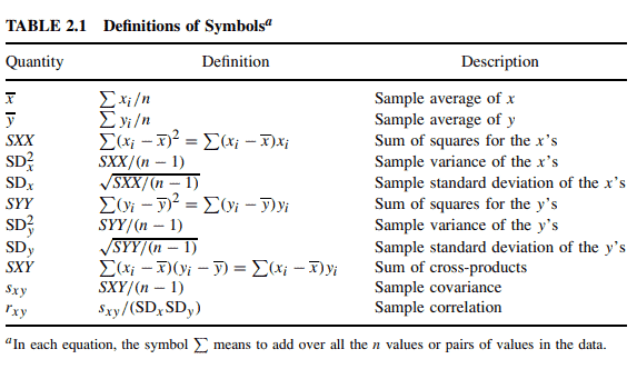
All least squares computations for simple regression depend only on averages, sums of squares and sums of cross-products. Definitions of the quantities used are given in Table 2.1. Sums of squares and cross-products have been centered by subtracting the average from each of the values before squaring or taking cross-products. Appropriate alternative formulas for computing the corrected sums of squares and cross products from uncorrected sums of squares and crossproducts that are often given in elementary textbooks are useful for mathematical proofs, but they can be highly inaccurate when used on a computer and should be avoided.
统计代写|线性回归代写Linear Regression代考|LEAST SQUARES CRITERION
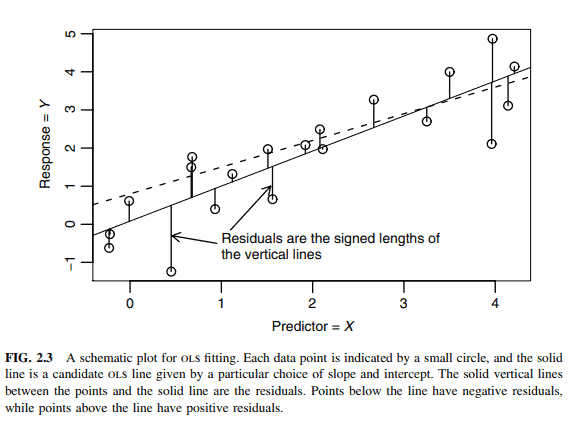
The criterion function for obtaining estimators is based on the residuals, which geometrically are the vertical distances between the fitted line and the actual $y$ values, as illustrated in Figure 2.3. The residuals reflect the inherent asymmetry in the roles of the response and the predictor in regression problems.
The oLs estimators are those values $\beta_0$ and $\beta_1$ that minimize the function ${ }^1$
$$
\operatorname{RSS}\left(\beta_0, \beta_1\right)=\sum_{i=1}^n\left[y_i-\left(\beta_0+\beta_1 x_i\right)\right]^2
$$
When evaluated at $\left(\hat{\beta}_0, \hat{\beta}_1\right)$, we call the quantity $\operatorname{RSS}\left(\hat{\beta}_0, \hat{\beta}_1\right)$ the residual sum of squares, or just $R S S$.
The least squares estimates can be derived in many ways, one of which is outlined in Appendix A.3. They are given by the expressions
$$
\begin{aligned}
& \hat{\beta}1=\frac{S X Y}{S X X}=r{x y} \frac{\mathrm{SD}y}{\mathrm{SD}_x}=r{x y}\left(\frac{S Y Y}{S X X}\right)^2 \
& \hat{\beta}_0=\bar{y}-\hat{\beta}_1 \bar{x}
\end{aligned}
$$
The several forms for $\hat{\beta}_1$ are all equivalent.
We emphasize again that oLs produces estimates of parameters but not the actual values of the parameters. The data in Figure 2.3 were created by setting the $x_i$ to be random sample of 20 numbers from a $\mathrm{N}(2,1.5)$ distribution and then computing $y_i=0.7+0.8 x_i+e_i$, where the errors were $\mathrm{N}(0,1)$ random numbers. For this graph, the true values of $\beta_0=0.7$ and $\beta_1=0.8$ are known. The graph of the true mean function is shown in Figure 2.3 as a dashed line, and it seems to match the data poorly compared to ols, given by the solid line. Since ols minimizes (2.4), it will always fit at least as well as, and generally better than, the true mean function.
Using Forbes’ data, we will write $\bar{x}$ to be the sample mean of Temp and $\bar{y}$ to be the sample mean of Lpres. The quantities needed for computing the least squares estimators are
$$
\begin{array}{lll}
\bar{x}=202.95294 & S X X=530.78235 & S X Y=475.31224 \
\bar{y}=139.60529 & S Y Y=427.79402 &
\end{array}
$$
The quantity $S Y Y$, although not yet needed, is given for completeness. In the rare instances that regression calculations are not done using statistical software or a statistical calculator, intermediate calculations such as these should be done as accurately as possible, and rounding should be done only to final results. Using (2.6), we find
$$
\begin{aligned}
& \hat{\beta}_1=\frac{S X Y}{S X X}=0.895 \
& \hat{\beta}_0=\bar{y}-\hat{\beta}_1 \bar{x}=-42.138
\end{aligned}
$$
线性回归代写
统计代写|线性回归代写Linear Regression代考|ORDINARY LEAST SQUARES ESTIMATION
已经提出了许多方法来获得模型中参数的估计。这里讨论的方法称为普通最小二乘法(oLs),其中选择参数估计来最小化称为残差平方和的量。附录A.3给出了最小二乘估计的正式发展。
参数是表征模型的未知量。参数的估计是数据的可计算函数,因此是统计。为了保持这种区分清晰,参数用$\alpha, \beta, \gamma$和$\sigma$这样的希腊字母表示,参数的估计通过在相应的希腊字母上加上一个“帽子”来表示。例如,$\hat{\beta}_1$(读作“beta 1 hat”)是$\beta_1$的估计量,$\hat{\sigma}^2$是$\sigma^2$的估计量。情况$i$的拟合值由$\widehat{\mathrm{E}}\left(Y \mid X=x_i\right)$给出,我们使用速记符号$\hat{y}_i$,
$$
\hat{y}_i=\widehat{\mathrm{E}}\left(Y \mid X=x_i\right)=\hat{\beta}_0+\hat{\beta}_1 x_i
$$
虽然$e_i$不是通常意义上的参数,但我们将使用相同的符号来指定残差:$i$第1种情况的残差记为$\hat{e}_i$,由方程
$$
\hat{e}_i=y_i-\widehat{\mathrm{E}}\left(Y \mid X=x_i\right)=y_i-\hat{y}_i=y_i-\left(\hat{\beta}_0+\hat{\beta}_1\right) \quad i=1, \ldots, n
$$
给出,该方程应与统计误差方程
$$
e_i=y_i-\left(\beta_0+\beta_1 x_i\right) \quad i=1, \ldots, n
$$
进行比较,简单回归的所有最小二乘计算仅依赖于平均值、平方和和叉乘和。所用数量的定义见表2.1。平方和和外积通过在平方或外积之前减去每个值的平均值来居中。从未校正的平方和和外积中计算校正的平方和和外积的适当的替代公式在数学证明中是有用的,但在计算机上使用时可能非常不准确,应避免使用。
统计代写|线性回归代写Linear Regression代考|LEAST SQUARES CRITERION
获得估计量的准则函数基于残差,残差在几何上是拟合线与实际$y$值之间的垂直距离,如图2.3所示。残差反映了响应和预测因子在回归问题中的作用的固有不对称性。
oLs估计量是那些使函数${ }^1$最小的值$\beta_0$和$\beta_1$
$$
\operatorname{RSS}\left(\beta_0, \beta_1\right)=\sum_{i=1}^n\left[y_i-\left(\beta_0+\beta_1 x_i\right)\right]^2
$$
当在$\left(\hat{\beta}_0, \hat{\beta}_1\right)$处求值时,我们称这个量$\operatorname{RSS}\left(\hat{\beta}_0, \hat{\beta}_1\right)$为残差平方和,或者简称为$R S S$。
最小二乘估计可以通过多种方式推导,附录A.3概述了其中一种方法。它们由表达式给出
$$
\begin{aligned}
& \hat{\beta}1=\frac{S X Y}{S X X}=r{x y} \frac{\mathrm{SD}y}{\mathrm{SD}_x}=r{x y}\left(\frac{S Y Y}{S X X}\right)^2 \
& \hat{\beta}_0=\bar{y}-\hat{\beta}_1 \bar{x}
\end{aligned}
$$
$\hat{\beta}_1$的几种形式都是等效的。
我们再次强调,oLs产生的是参数的估计,而不是参数的实际值。图2.3中的数据是这样创建的:将$x_i$设置为来自$\mathrm{N}(2,1.5)$分布的20个数字的随机样本,然后计算$y_i=0.7+0.8 x_i+e_i$,其中误差为$\mathrm{N}(0,1)$随机数。对于这个图,$\beta_0=0.7$和$\beta_1=0.8$的真实值是已知的。真实均值函数的图形如图2.3所示为虚线,与实线给出的ols相比,它似乎与数据匹配得很差。由于ols最小化(2.4),它总是至少与真实均值函数一样适合,并且通常比真实均值函数更好。
使用福布斯的数据,我们将$\bar{x}$作为Temp的样本均值,$\bar{y}$作为Lpres的样本均值。计算最小二乘估计量所需的量是
$$
\begin{array}{lll}
\bar{x}=202.95294 & S X X=530.78235 & S X Y=475.31224 \
\bar{y}=139.60529 & S Y Y=427.79402 &
\end{array}
$$
虽然还不需要,但为了完整起见,给出了$S Y Y$这个数量。在不使用统计软件或统计计算器进行回归计算的极少数情况下,应该尽可能准确地进行诸如此类的中间计算,并且应该只对最终结果进行舍入。使用(2.6),我们发现
$$
\begin{aligned}
& \hat{\beta}_1=\frac{S X Y}{S X X}=0.895 \
& \hat{\beta}_0=\bar{y}-\hat{\beta}_1 \bar{x}=-42.138
\end{aligned}
$$

统计代写|线性回归代写Linear Regression代考 请认准UprivateTA™. UprivateTA™为您的留学生涯保驾护航。
微观经济学代写
微观经济学是主流经济学的一个分支,研究个人和企业在做出有关稀缺资源分配的决策时的行为以及这些个人和企业之间的相互作用。my-assignmentexpert™ 为您的留学生涯保驾护航 在数学Mathematics作业代写方面已经树立了自己的口碑, 保证靠谱, 高质且原创的数学Mathematics代写服务。我们的专家在图论代写Graph Theory代写方面经验极为丰富,各种图论代写Graph Theory相关的作业也就用不着 说。
线性代数代写
线性代数是数学的一个分支,涉及线性方程,如:线性图,如:以及它们在向量空间和通过矩阵的表示。线性代数是几乎所有数学领域的核心。
博弈论代写
现代博弈论始于约翰-冯-诺伊曼(John von Neumann)提出的两人零和博弈中的混合策略均衡的观点及其证明。冯-诺依曼的原始证明使用了关于连续映射到紧凑凸集的布劳威尔定点定理,这成为博弈论和数学经济学的标准方法。在他的论文之后,1944年,他与奥斯卡-莫根斯特恩(Oskar Morgenstern)共同撰写了《游戏和经济行为理论》一书,该书考虑了几个参与者的合作游戏。这本书的第二版提供了预期效用的公理理论,使数理统计学家和经济学家能够处理不确定性下的决策。
微积分代写
微积分,最初被称为无穷小微积分或 “无穷小的微积分”,是对连续变化的数学研究,就像几何学是对形状的研究,而代数是对算术运算的概括研究一样。
它有两个主要分支,微分和积分;微分涉及瞬时变化率和曲线的斜率,而积分涉及数量的累积,以及曲线下或曲线之间的面积。这两个分支通过微积分的基本定理相互联系,它们利用了无限序列和无限级数收敛到一个明确定义的极限的基本概念 。
计量经济学代写
什么是计量经济学?
计量经济学是统计学和数学模型的定量应用,使用数据来发展理论或测试经济学中的现有假设,并根据历史数据预测未来趋势。它对现实世界的数据进行统计试验,然后将结果与被测试的理论进行比较和对比。
根据你是对测试现有理论感兴趣,还是对利用现有数据在这些观察的基础上提出新的假设感兴趣,计量经济学可以细分为两大类:理论和应用。那些经常从事这种实践的人通常被称为计量经济学家。
Matlab代写
MATLAB 是一种用于技术计算的高性能语言。它将计算、可视化和编程集成在一个易于使用的环境中,其中问题和解决方案以熟悉的数学符号表示。典型用途包括:数学和计算算法开发建模、仿真和原型制作数据分析、探索和可视化科学和工程图形应用程序开发,包括图形用户界面构建MATLAB 是一个交互式系统,其基本数据元素是一个不需要维度的数组。这使您可以解决许多技术计算问题,尤其是那些具有矩阵和向量公式的问题,而只需用 C 或 Fortran 等标量非交互式语言编写程序所需的时间的一小部分。MATLAB 名称代表矩阵实验室。MATLAB 最初的编写目的是提供对由 LINPACK 和 EISPACK 项目开发的矩阵软件的轻松访问,这两个项目共同代表了矩阵计算软件的最新技术。MATLAB 经过多年的发展,得到了许多用户的投入。在大学环境中,它是数学、工程和科学入门和高级课程的标准教学工具。在工业领域,MATLAB 是高效研究、开发和分析的首选工具。MATLAB 具有一系列称为工具箱的特定于应用程序的解决方案。对于大多数 MATLAB 用户来说非常重要,工具箱允许您学习和应用专业技术。工具箱是 MATLAB 函数(M 文件)的综合集合,可扩展 MATLAB 环境以解决特定类别的问题。可用工具箱的领域包括信号处理、控制系统、神经网络、模糊逻辑、小波、仿真等。