如果你也在 怎样代写回归分析Regression Analysis 这个学科遇到相关的难题,请随时右上角联系我们的24/7代写客服。回归分析Regression Analysis被广泛用于预测和预报,其使用与机器学习领域有很大的重叠。在某些情况下,回归分析可以用来推断自变量和因变量之间的因果关系。重要的是,回归本身只揭示了固定数据集中因变量和自变量集合之间的关系。为了分别使用回归进行预测或推断因果关系,研究者必须仔细论证为什么现有的关系对新的环境具有预测能力,或者为什么两个变量之间的关系具有因果解释。当研究者希望使用观察数据来估计因果关系时,后者尤其重要。
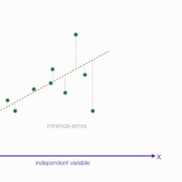
回归分析Regression Analysis在统计建模中,回归分析是一组统计过程,用于估计因变量(通常称为 “结果 “或 “响应 “变量,或机器学习术语中的 “标签”)与一个或多个自变量(通常称为 “预测因子”、”协变量”、”解释变量 “或 “特征”)之间的关系。回归分析最常见的形式是线性回归,即根据特定的数学标准找到最适合数据的直线(或更复杂的线性组合)。例如,普通最小二乘法计算唯一的直线(或超平面),使真实数据与该直线(或超平面)之间的平方差之和最小。由于特定的数学原因(见线性回归),这使得研究者能够在自变量具有一组给定值时估计因变量的条件期望值(或人口平均值)。不太常见的回归形式使用稍微不同的程序来估计替代位置参数(例如,量化回归或必要条件分析),或在更广泛的非线性模型集合中估计条件期望值(例如,非参数回归)。
回归分析Regression Analysis代写,免费提交作业要求, 满意后付款,成绩80\%以下全额退款,安全省心无顾虑。专业硕 博写手团队,所有订单可靠准时,保证 100% 原创。 最高质量的回归分析Regression Analysis作业代写,服务覆盖北美、欧洲、澳洲等 国家。 在代写价格方面,考虑到同学们的经济条件,在保障代写质量的前提下,我们为客户提供最合理的价格。 由于作业种类很多,同时其中的大部分作业在字数上都没有具体要求,因此回归分析Regression Analysis作业代写的价格不固定。通常在专家查看完作业要求之后会给出报价。作业难度和截止日期对价格也有很大的影响。
同学们在留学期间,都对各式各样的作业考试很是头疼,如果你无从下手,不如考虑my-assignmentexpert™!
my-assignmentexpert™提供最专业的一站式服务:Essay代写,Dissertation代写,Assignment代写,Paper代写,Proposal代写,Proposal代写,Literature Review代写,Online Course,Exam代考等等。my-assignmentexpert™专注为留学生提供Essay代写服务,拥有各个专业的博硕教师团队帮您代写,免费修改及辅导,保证成果完成的效率和质量。同时有多家检测平台帐号,包括Turnitin高级账户,检测论文不会留痕,写好后检测修改,放心可靠,经得起任何考验!
想知道您作业确定的价格吗? 免费下单以相关学科的专家能了解具体的要求之后在1-3个小时就提出价格。专家的 报价比上列的价格能便宜好几倍。
我们在统计Statistics代写方面已经树立了自己的口碑, 保证靠谱, 高质且原创的统计Statistics代写服务。我们的专家在回归分析Regression Analysis代写方面经验极为丰富,各种回归分析Regression Analysis相关的作业也就用不着 说。
统计代写|回归分析代写Regression Analysis代考|Randomness of the Measured Area of a Circle as Related to Its Measured Radius
A circle in nature has its radius $(X)$ measured. Suppose the measurement is $X=10$ meters. Still, there are many potentially observable measurements of its area, $Y$, due to imperfections in the circle and imperfections in the measuring device. The regression model states that $Y$ is a random observation from the conditional distribution $p(y \mid X=10)$.
This model is reasonable, because it perfectly matches the reality that there are many potentially observable measurements of the area $Y$, even when the radius $X$ is measured to be precisely 10 meters. Note that this model does not say anything about the mean of the distribution $p(y \mid x)$ : It might be $3.14159265 x^2$, but it is more likely not, because of biases in the data-generating process (again, this data-generating process includes imperfections in circles, and also imperfections in the measuring devices).
This model also does not say anything about the nature of the probability distributions $p(y \mid x)$, whether they are discrete, continuous, normal, lognormal, etc., or even whether you have one type of distribution for one $x$ (e.g., normal) and another for a different $x$ (e.g., Poisson). It simply says there is a distribution $p(y \mid x)$ of potential outcomes of $Y$ when $X=x$, and that the number you measure will appear as if produced at random from this distribution, i.e., as if simulated using a random number generator. As such, there is no arguing with the model-the measured data really will look this way (random, variable), hence you may even say that this model is a correct model because it produces data that are random and variable (non-deterministic). Further, because the model is so general, no data can ever contradict, or “reject” it.
Thus, the model $p(y \mid x)$ is correct. It is only when you make assumptions about the nature of $p(y \mid x)$, for example, about the specific distributions (e.g. normal), and about how are distributions related to $x$ (e.g., linearly), that you must consider that the model is wrong in certain ways.
The model $p(y \mid x)$ does not require that the distribution of $Y$ change for different values of $X$. If the distributions $p(y \mid x)$ are the same, for all values $X=x$, then, by definition, $Y$ is independent of $X$. In the example above, one may logically assume that the distributions of $Y$ (measured area) will differ greatly for different $X$ (measured radius), and that $Y$ and $X$ are thus strongly dependent.
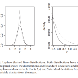
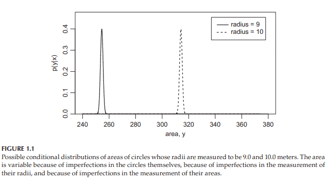
The following R code and resulting graph of Figure 1.1 illustrate how the distributions of area $(Y)$ might look for circles whose radius $(X)$ is measured to be 9.0 meters versus circles whose radius is measured to be 10.0 meters. In this example, we assume that $p(y \mid x)$ is a normal distribution with mean $\pi x^2$ meters ${ }^2$ and standard deviation of 1 meter $^2$
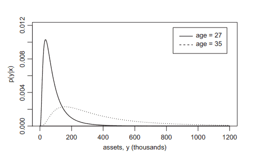
统计代写|回归分析代写Regression Analysis代考|Randomness of a Person’s Financial Assets as Related to Their Age
Can you predict a person’s financial assets from their age? Suppose you know that a person’s age is $X=27$ years, but you know nothing else about that person. The regression model states that the person’s assets, $Y$, comes from a distribution $p(y \mid X=27)$.
Again, this model also does not say anything about the nature of the distributions $p(y \mid x)$, whether they are discrete, continuous, normal, lognormal, etc. It simply says that, for a particular value of Age $(x)$, there is a distribution of potential assets, and that the assets of a particular person having Age $=x$ can be viewed as a number produced at random from this distribution, as if simulated using a random number generator. As such, there is no arguing with the model-the assets data really do look this way (variable), hence this model is correct. Again, it is only when you make assumptions about the nature of $p(y \mid x)$, for example, what is the specific distribution (e.g., normal), and how are distributions related to $x$ (e.g., linearly), that you must acknowledge that the model is “wrong” in certain ways.
The regression models $p(y \mid x)$ assumed in the following code are “lognormal” probability distributions, chosen this way because assets are non-negative, and because lognormal distributions (among many other distributions) can be used to model non-negative observations. (Normal distributions can also be used to model non-negative observations, provided that the tail area to the left of zero is very small, as in Figure 1.1) But lognormal distributions are used for illustration only. The general regression model $p(y \mid x)$ makes no assumption about the nature of the distributions.
回归分析代写
统计代写|回归分析代写Regression Analysis代考|Introduction to Regression Models
回归模型用于将变量$Y$与单个变量$X$或多个变量联系起来,$X_1, X_2, \ldots, X_k$ .
这里有一些例子,这些模型可以帮助你回答的问题:
一个人的牙膏选择$(Y)$与这个人的年龄$\left(X_1\right)$和收入$\left(X_2\right)$有什么关系?
一个人的癌症缓解状态$(Y)$与他们的化疗方案有什么关系$(X)$ ?
道路上坑洼的数量$(Y)$与路面使用的材料$\left(X_1\right)$和安装后的时间有什么关系$\left(X_2\right)$ ?
一个人偿还贷款的能力$(Y)$与这个人的收入$\left(X_1\right)$、资产$\left(X_2\right)$、和$\operatorname{debt}\left(X_3\right)$ ?
一个人购买技术产品的意图$(Y)$与他们感知到的有用性$\left(X_1\right)$和感知到的产品易用性$\left(X_2\right)$有什么关系?
今天标普500指数的回报$(Y)$与昨天的回报有什么关系$(X) ?$
一家公司的盈利能力$(Y)$与它在质量管理方面的投资有什么关系$(X)$ ?
理解这些关系可以帮助你预测对于给定的固定值$X$,未知的$Y$会是什么样子,它可以帮助你决定你应该选择什么样的行动方针,它可以帮助你以科学的方式理解你正在学习的科目。回归模型也可以帮助你预测未来。预测是预测的一种特殊情况:预测意味着对未来的预测,而预测包括任何类型的“假设”分析,不仅是关于未来可能发生的事情,而且还包括过去在不同情况下可能发生的事情。
在某些科目中,您将学习使用诸如
$$
Y=f(X)
$$
等方程进行预测,其中函数$f$可能是线性,二次,指数或对数函数;或者它可能根本没有任何“命名”函数形式。但是,在所有情况下,这都是一种确定性关系:给定变量$X$的特定值$x$, $Y$的值完全由$Y=f(x)$决定。
统计代写|回归分析代写Regression Analysis代考|The Regression Model in Terms of Conditional Distributions
回归模型假设数据值$Y$来自不同的分布,其中对于一般变量$X$的每个特定值$x$都有不同的分布。这个模型用符号表示如下:
回归模型
$$
Y \mid X=x \sim p(y \mid x)
$$
表达式$p(y \mid X=x)$是$X=x$时潜在可观察到的$Y$值的分布,它被称为$Y$的条件分布,假设$X=x$。有时为了简洁起见,这些条件分布将写成$p(y \mid x)$。
下面的例子阐明了这个抽象。
自然界中圆的半径$(X)$是测量出来的。假设测量值是$X=10$米。尽管如此,由于圆和测量装置的缺陷,它的面积仍有许多潜在的可观察到的测量值$Y$。回归模型表明$Y$是条件分布$p(y \mid X=10)$的随机观测值。
这个模型是合理的,因为它完全符合现实,即有许多潜在的可观察到的面积$Y$,即使半径$X$被精确测量为10米。请注意,这个模型并没有说明$p(y \mid x)$分布的平均值:它可能是$3.14159265 x^2$,但更有可能不是,因为数据生成过程中的偏差(再次,这个数据生成过程包括圆圈中的缺陷,以及测量设备中的缺陷)。
这个模型也没有说任何关于概率分布$p(y \mid x)$的性质,无论它们是离散的,连续的,正态的,对数正态的,等等,或者你是否有一种类型的分布$x$(例如,正态)和另一种类型的分布$x$(例如,泊松)。它简单地说,当$X=x$时,存在一个潜在结果$Y$的分布$p(y \mid x)$,并且您测量的数字将看起来像是从该分布随机产生的,也就是说,好像使用随机数生成器模拟。因此,模型是没有争议的——测量的数据确实是这样的(随机的,可变的),因此你甚至可以说这个模型是一个正确的模型,因为它产生的数据是随机的和可变的(非确定性的)。此外,由于模型是如此普遍,没有任何数据可以反驳或“拒绝”它。

统计代写|回归分析代写Regression Analysis代考 请认准UprivateTA™. UprivateTA™为您的留学生涯保驾护航。
微观经济学代写
微观经济学是主流经济学的一个分支,研究个人和企业在做出有关稀缺资源分配的决策时的行为以及这些个人和企业之间的相互作用。my-assignmentexpert™ 为您的留学生涯保驾护航 在数学Mathematics作业代写方面已经树立了自己的口碑, 保证靠谱, 高质且原创的数学Mathematics代写服务。我们的专家在图论代写Graph Theory代写方面经验极为丰富,各种图论代写Graph Theory相关的作业也就用不着 说。
线性代数代写
线性代数是数学的一个分支,涉及线性方程,如:线性图,如:以及它们在向量空间和通过矩阵的表示。线性代数是几乎所有数学领域的核心。
博弈论代写
现代博弈论始于约翰-冯-诺伊曼(John von Neumann)提出的两人零和博弈中的混合策略均衡的观点及其证明。冯-诺依曼的原始证明使用了关于连续映射到紧凑凸集的布劳威尔定点定理,这成为博弈论和数学经济学的标准方法。在他的论文之后,1944年,他与奥斯卡-莫根斯特恩(Oskar Morgenstern)共同撰写了《游戏和经济行为理论》一书,该书考虑了几个参与者的合作游戏。这本书的第二版提供了预期效用的公理理论,使数理统计学家和经济学家能够处理不确定性下的决策。
微积分代写
微积分,最初被称为无穷小微积分或 “无穷小的微积分”,是对连续变化的数学研究,就像几何学是对形状的研究,而代数是对算术运算的概括研究一样。
它有两个主要分支,微分和积分;微分涉及瞬时变化率和曲线的斜率,而积分涉及数量的累积,以及曲线下或曲线之间的面积。这两个分支通过微积分的基本定理相互联系,它们利用了无限序列和无限级数收敛到一个明确定义的极限的基本概念 。
计量经济学代写
什么是计量经济学?
计量经济学是统计学和数学模型的定量应用,使用数据来发展理论或测试经济学中的现有假设,并根据历史数据预测未来趋势。它对现实世界的数据进行统计试验,然后将结果与被测试的理论进行比较和对比。
根据你是对测试现有理论感兴趣,还是对利用现有数据在这些观察的基础上提出新的假设感兴趣,计量经济学可以细分为两大类:理论和应用。那些经常从事这种实践的人通常被称为计量经济学家。
Matlab代写
MATLAB 是一种用于技术计算的高性能语言。它将计算、可视化和编程集成在一个易于使用的环境中,其中问题和解决方案以熟悉的数学符号表示。典型用途包括:数学和计算算法开发建模、仿真和原型制作数据分析、探索和可视化科学和工程图形应用程序开发,包括图形用户界面构建MATLAB 是一个交互式系统,其基本数据元素是一个不需要维度的数组。这使您可以解决许多技术计算问题,尤其是那些具有矩阵和向量公式的问题,而只需用 C 或 Fortran 等标量非交互式语言编写程序所需的时间的一小部分。MATLAB 名称代表矩阵实验室。MATLAB 最初的编写目的是提供对由 LINPACK 和 EISPACK 项目开发的矩阵软件的轻松访问,这两个项目共同代表了矩阵计算软件的最新技术。MATLAB 经过多年的发展,得到了许多用户的投入。在大学环境中,它是数学、工程和科学入门和高级课程的标准教学工具。在工业领域,MATLAB 是高效研究、开发和分析的首选工具。MATLAB 具有一系列称为工具箱的特定于应用程序的解决方案。对于大多数 MATLAB 用户来说非常重要,工具箱允许您学习和应用专业技术。工具箱是 MATLAB 函数(M 文件)的综合集合,可扩展 MATLAB 环境以解决特定类别的问题。可用工具箱的领域包括信号处理、控制系统、神经网络、模糊逻辑、小波、仿真等。