如果你也在 怎样代写回归分析Regression Analysis 这个学科遇到相关的难题,请随时右上角联系我们的24/7代写客服。回归分析Regression Analysis是一种显示两个或多个变量之间关系的统计方法。通常用图表表示,该方法检验因变量与自变量之间的关系。通常,自变量随因变量而变化,回归分析试图回答哪些因素对这种变化最重要。
回归分析Regression Analysis中的预测可以涵盖各种各样的情况和场景。例如,预测有多少人会看到广告牌可以帮助管理层决定投资广告是否是个好主意;在哪种情况下,这个广告牌能提供良好的投资回报?保险公司和银行大量使用回归分析的预测。有多少抵押贷款持有人会按时偿还贷款?有多少投保人会遭遇车祸或家中被盗?这些预测允许进行风险评估,但也可以预测最佳费用和溢价。
回归分析Regression Analysis代写,免费提交作业要求, 满意后付款,成绩80\%以下全额退款,安全省心无顾虑。专业硕 博写手团队,所有订单可靠准时,保证 100% 原创。 最高质量的回归分析Regression Analysis作业代写,服务覆盖北美、欧洲、澳洲等 国家。 在代写价格方面,考虑到同学们的经济条件,在保障代写质量的前提下,我们为客户提供最合理的价格。 由于作业种类很多,同时其中的大部分作业在字数上都没有具体要求,因此回归分析Regression Analysis作业代写的价格不固定。通常在专家查看完作业要求之后会给出报价。作业难度和截止日期对价格也有很大的影响。
同学们在留学期间,都对各式各样的作业考试很是头疼,如果你无从下手,不如考虑my-assignmentexpert™!
my-assignmentexpert™提供最专业的一站式服务:Essay代写,Dissertation代写,Assignment代写,Paper代写,Proposal代写,Proposal代写,Literature Review代写,Online Course,Exam代考等等。my-assignmentexpert™专注为留学生提供Essay代写服务,拥有各个专业的博硕教师团队帮您代写,免费修改及辅导,保证成果完成的效率和质量。同时有多家检测平台帐号,包括Turnitin高级账户,检测论文不会留痕,写好后检测修改,放心可靠,经得起任何考验!
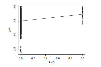
统计代写|回归分析代写Regression Analysis代考|Does It Matter Whether the Indicator Variable Is Coded as 1,0 vs. 0,1 ?
It does not matter in the sense that you can code it either way; neither is preferred. It does matter in the sense that the parameter interpretations will all be reversed. If you code Master’s as 1 and $\mathrm{PhD}$ as 0 , then $\beta_0$ becomes the mean for $\mathrm{PhD}$ students, and $\beta_1$ is the difference between Master’s mean and PhD mean. Here is the output:
Coefficients:
$\begin{array}{lrrrr} & \text { Estimate } & \text { Std. Error } t \text { value } \operatorname{Pr}(>|t|) \ \text { (Intercept) } & 3.73631 & 0.04937 & 75.676<2 e-16 \star \star * \ \text { Masters } & -0.24010 & 0.05128 & -4.682 & 3.67 e-06 \star * *\end{array}$
Now, the intercept 3.73631 is the mean of the observed GPA for PhD students, and the difference between Master’s and PhD means is -0.24010 . It’s exactly the same information as before, just labeled differently. Further, using the confint function, you get $-0.3408432<\beta_1<-0.1393487$, meaning that the mean of potentially observable GPAs for Master’s students is somewhere between 0.1393487 and 0.3408432 lower than the mean of potentially observable GPAs for $\mathrm{PhD}$ students. Again, this information is exactly as before, just from a different point of view.
The analysis above that compares Master’s and PhD students is identical to the twosample $t$ test, which we hope you have seen in a prior course. In R, you can perform the two-sample $t$ test as follows:
t.test (gpa $\sim$ degree, var. equal=T)
The output provides identical $|T|$ statistic and confidence interval as the regression analysis:
Two Sample t-test
data: gpa by degree
$t=-4.6824, \mathrm{df}=492, \mathrm{p}$-value $=3.672 \mathrm{e}-06$
alternative hypothesis: true difference in means is not equal to 0
95 percent confidence interval:
$-0.3408432-0.1393487$
sample estimates:
mean in group $M$ mean in group $P$
3.496210
736306
统计代写|回归分析代写Regression Analysis代考|Using Multiple Indicator Variables to Represent a Single Nominal Variable Having Three or More Levels (ANOVA)
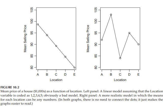
“Location, location, location!” is what the real estate folks tell you. The price of a home is strongly affected by where the house is located.
Consider the following data set on house prices.
house $=$ read.csv (“https://raw.githubusercontent. com/andrea2719/
URA-Datasets/master/house.csv”, header=T) ; attach (house)
Two variables in the data set are “sell” and “location”; respectively the selling price (in $\$ 1,000 s)$ of a home, and its location. The “Location” variable has five levels, either location A, B, C, D, or E.
Whenever you have a nominal variable, you should always check the sample sizes within all of the levels, because small sample sizes will give imprecise estimates. By entering the command table(location), you get the following result:
\begin{tabular}{rrrrr}
\multicolumn{4}{c}{ location } \
A & B & C & D & E \
26 & 15 & 4 & 9 & 10
\end{tabular}
Notice that there are only 4 homes in location “C.” Thus, the average of potentially observable house price in location $\mathrm{C}$ is estimated less accurately than it is in the other locations.
The goal is to model $Y \mid X=x$, selling price of a home, as a function of $X$, location. As always in regression, you will specify a model $p(y \mid X=x)$ for every $X=x$; which, in this case, means you need to specify the models $p(y \mid X=A), p(y \mid X=B), p(y \mid X=C), p(y \mid X=D)$, and $p(y \mid X=E)$.
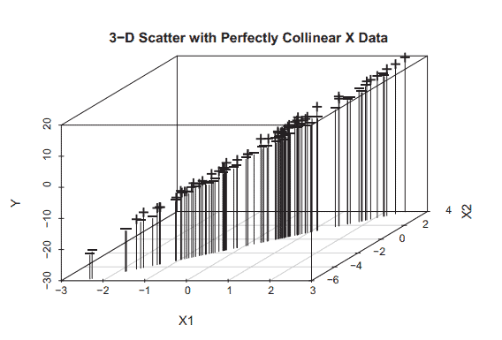
A problem is that location is character data (A, B, C, D, and E). You cannot use the classical regression model to specify these distributions, because that model states that the means of the distributions are a linear function of $X=x$, and here, the specific values of $X$ are not numbers, they are letters. You might consider recoding the locations as a new variable $U$, where $U=1$ for location $\mathrm{A}, U=2$, for location $\mathrm{B}, \ldots, U=5$ for location $\mathrm{E}$, and then perform the regression of $Y$ on $U$, but that would presume a perfect linear function of mean values for the different locations. This really makes no sense at all-the locations are not even ordinal, in the sense that A is somehow “less than” B, which is in turn “less than” C, and so forth. Rather, they are just five locations, and the mean selling prices could be anything for each location, with no connection (linear or otherwise) between the means for different locations. Figure 10.2 shows graphs of the mean function assuming such a $U$ variable, and the more realistic case where the mean selling prices can be any numbers.
So, how do you model “Location” so that the mean selling price can be anything at all in each location, as shown in the right panel of Figure 10.2? Simple. Define four indicator variables for the locations, leaving one out. Specifically, let:
$$
\begin{aligned}
& X A=1 \text { if location } A, 0 \text { otherwise } \
& X B=1 \text { if location } B, 0 \text { otherwise } \
& X C=1 \text { if location } C, 0 \text { otherwise } \
& X D=1 \text { if location } D, 0 \text { otherwise }
\end{aligned}
$$
回归分析代写
统计代写|回归分析代写Regression Analysis代考|Does It Matter Whether the Indicator Variable Is Coded as 1,0 vs. 0,1 ?
这并不重要,因为你可以用任何一种方式来编码;两者都不是首选。在参数解释全部颠倒的意义上,它确实很重要。如果将Master’s编码为1,将$\mathrm{PhD}$编码为0,则$\beta_0$成为$\mathrm{PhD}$学生的平均值,而$\beta_1$是Master’s平均值和PhD ‘s平均值之间的差值。输出如下:
系数:
$\begin{array}{lrrrr} & \text {Estimate} & \text {Std. Error} t \text {value} \operatorname{Pr}(>|t|) \ \text {(Intercept)} & 3.73631 & 0.04937 & 75.676<2 e-16 \star \star *\ text {Masters} & -0.24010 & 0.05128 & -4.682 & 3.67 e-06 \star * *\end{array}$
现在,截距3.73631是博士生观察到的GPA的平均值,硕士和博士的平均值之差是-0.24010。它和之前的信息完全一样,只是标记不同。此外,使用约束函数,你得到$-0.3408432<\beta_1<-0.1393487$,这意味着硕士生的潜在可观察gpa的平均值比$\ mathm {PhD}$学生的潜在可观察gpa的平均值低0.1393487和0.3408432。同样,这个信息和之前完全一样,只是从不同的角度来看。
上面比较硕士和博士学生的分析与两样本t测试相同,我们希望您在之前的课程中看到过。在R中,您可以执行以下两样本$t$检验:
T .test (gpa $\sim$ degree, var. equal=T)
输出提供与回归分析相同的$|T|$统计量和置信区间:
双样本t检验
数据:按学位计算的gpa
t = -4.6824美元,\ mathrm {df} = 492, \ mathrm {p}值= 3.672美元\ mathrm {e} -06美元
备择假设:真均值差不等于0
95%置信区间:
-0.3408432 – -0.1393487美元
样本估计:
M组的平均值P组的平均值
3.496210
736306
统计代写|回归分析代写Regression Analysis代考|Using Multiple Indicator Variables to Represent a Single Nominal Variable Having Three or More Levels (ANOVA)
“地段,地段,地段!”这是房地产商告诉你的。房子的位置对房价有很大影响。
考虑下面的房价数据集。
House $=$ read.csv (“https://raw.githubusercontent。com/andrea2719/
URA-Datasets/master/house.csv”, header=T);随员(屋宇)
数据集中的两个变量是“sell”和“location”;分别是房屋的售价(网址:$\$ 1,000 s)$)和位置。“Location”变量有五个级别,分别是位置A、B、C、D或E。
当你有一个名义变量时,你应该总是检查所有水平内的样本大小,因为小的样本大小会给出不精确的估计。通过输入命令表(location),可以得到以下结果:
\begin{tabular}{rrrrr}
\multicolumn{4}{c}{ location } \A & B & C & D & E\26 & 15 & 4 & 9 & 10\end{tabular}
注意位置c只有4户人家因此,位置$\mathrm{C}$的潜在可观察房价的平均值估计不如其他位置准确。
目标是将房屋售价$Y \mid X=x$作为位置$X$的函数进行建模。在回归中,您将为每个$X=x$指定一个模型$p(y \mid X=x)$;在这种情况下,这意味着您需要指定模型$p(y \mid X=A), p(y \mid X=B), p(y \mid X=C), p(y \mid X=D)$和$p(y \mid X=E)$。
一个问题是,位置是字符数据(A、B、C、D和E)。您不能使用经典回归模型来指定这些分布,因为该模型表明分布的平均值是$X=x$的线性函数,在这里,$X$的特定值不是数字,而是字母。您可以考虑将位置重新编码为一个新变量$U$,其中$U=1$表示位置$\mathrm{A}, U=2$,对于位置$\mathrm{B}, \ldots, U=5$表示位置$\mathrm{E}$,然后对$U$执行$Y$的回归,但这将假设不同位置的平均值具有完美的线性函数。这完全没有意义——位置甚至不是有序的,从某种意义上说,A“小于”B,而B又“小于”C,以此类推。相反,它们只是五个地点,每个地点的平均销售价格可以是任何东西,不同地点的平均值之间没有联系(线性或其他)。图10.2显示了假设这样一个$U$变量的平均函数的图形,以及更现实的情况,即平均销售价格可以是任何数字。
那么,如何为“Location”建模,以便每个位置的平均销售价格可以是任意值,如图10.2的右面板所示?很简单。为位置定义四个指示器变量,省略一个。具体来说,让:
$$
\begin{aligned}
& X A=1 \text { if location } A, 0 \text { otherwise } \
& X B=1 \text { if location } B, 0 \text { otherwise } \
& X C=1 \text { if location } C, 0 \text { otherwise } \
& X D=1 \text { if location } D, 0 \text { otherwise }
\end{aligned}
$$

统计代写|回归分析代写Regression Analysis代考 请认准UprivateTA™. UprivateTA™为您的留学生涯保驾护航。
微观经济学代写
微观经济学是主流经济学的一个分支,研究个人和企业在做出有关稀缺资源分配的决策时的行为以及这些个人和企业之间的相互作用。my-assignmentexpert™ 为您的留学生涯保驾护航 在数学Mathematics作业代写方面已经树立了自己的口碑, 保证靠谱, 高质且原创的数学Mathematics代写服务。我们的专家在图论代写Graph Theory代写方面经验极为丰富,各种图论代写Graph Theory相关的作业也就用不着 说。
线性代数代写
线性代数是数学的一个分支,涉及线性方程,如:线性图,如:以及它们在向量空间和通过矩阵的表示。线性代数是几乎所有数学领域的核心。
博弈论代写
现代博弈论始于约翰-冯-诺伊曼(John von Neumann)提出的两人零和博弈中的混合策略均衡的观点及其证明。冯-诺依曼的原始证明使用了关于连续映射到紧凑凸集的布劳威尔定点定理,这成为博弈论和数学经济学的标准方法。在他的论文之后,1944年,他与奥斯卡-莫根斯特恩(Oskar Morgenstern)共同撰写了《游戏和经济行为理论》一书,该书考虑了几个参与者的合作游戏。这本书的第二版提供了预期效用的公理理论,使数理统计学家和经济学家能够处理不确定性下的决策。
微积分代写
微积分,最初被称为无穷小微积分或 “无穷小的微积分”,是对连续变化的数学研究,就像几何学是对形状的研究,而代数是对算术运算的概括研究一样。
它有两个主要分支,微分和积分;微分涉及瞬时变化率和曲线的斜率,而积分涉及数量的累积,以及曲线下或曲线之间的面积。这两个分支通过微积分的基本定理相互联系,它们利用了无限序列和无限级数收敛到一个明确定义的极限的基本概念 。
计量经济学代写
什么是计量经济学?
计量经济学是统计学和数学模型的定量应用,使用数据来发展理论或测试经济学中的现有假设,并根据历史数据预测未来趋势。它对现实世界的数据进行统计试验,然后将结果与被测试的理论进行比较和对比。
根据你是对测试现有理论感兴趣,还是对利用现有数据在这些观察的基础上提出新的假设感兴趣,计量经济学可以细分为两大类:理论和应用。那些经常从事这种实践的人通常被称为计量经济学家。
Matlab代写
MATLAB 是一种用于技术计算的高性能语言。它将计算、可视化和编程集成在一个易于使用的环境中,其中问题和解决方案以熟悉的数学符号表示。典型用途包括:数学和计算算法开发建模、仿真和原型制作数据分析、探索和可视化科学和工程图形应用程序开发,包括图形用户界面构建MATLAB 是一个交互式系统,其基本数据元素是一个不需要维度的数组。这使您可以解决许多技术计算问题,尤其是那些具有矩阵和向量公式的问题,而只需用 C 或 Fortran 等标量非交互式语言编写程序所需的时间的一小部分。MATLAB 名称代表矩阵实验室。MATLAB 最初的编写目的是提供对由 LINPACK 和 EISPACK 项目开发的矩阵软件的轻松访问,这两个项目共同代表了矩阵计算软件的最新技术。MATLAB 经过多年的发展,得到了许多用户的投入。在大学环境中,它是数学、工程和科学入门和高级课程的标准教学工具。在工业领域,MATLAB 是高效研究、开发和分析的首选工具。MATLAB 具有一系列称为工具箱的特定于应用程序的解决方案。对于大多数 MATLAB 用户来说非常重要,工具箱允许您学习和应用专业技术。工具箱是 MATLAB 函数(M 文件)的综合集合,可扩展 MATLAB 环境以解决特定类别的问题。可用工具箱的领域包括信号处理、控制系统、神经网络、模糊逻辑、小波、仿真等。