如果你也在 怎样代写回归分析Regression Analysis 这个学科遇到相关的难题,请随时右上角联系我们的24/7代写客服。回归分析Regression Analysis是一种显示两个或多个变量之间关系的统计方法。通常用图表表示,该方法检验因变量与自变量之间的关系。通常,自变量随因变量而变化,回归分析试图回答哪些因素对这种变化最重要。
回归分析Regression Analysis中的预测可以涵盖各种各样的情况和场景。例如,预测有多少人会看到广告牌可以帮助管理层决定投资广告是否是个好主意;在哪种情况下,这个广告牌能提供良好的投资回报?保险公司和银行大量使用回归分析的预测。有多少抵押贷款持有人会按时偿还贷款?有多少投保人会遭遇车祸或家中被盗?这些预测允许进行风险评估,但也可以预测最佳费用和溢价。
回归分析Regression Analysis代写,免费提交作业要求, 满意后付款,成绩80\%以下全额退款,安全省心无顾虑。专业硕 博写手团队,所有订单可靠准时,保证 100% 原创。 最高质量的回归分析Regression Analysis作业代写,服务覆盖北美、欧洲、澳洲等 国家。 在代写价格方面,考虑到同学们的经济条件,在保障代写质量的前提下,我们为客户提供最合理的价格。 由于作业种类很多,同时其中的大部分作业在字数上都没有具体要求,因此回归分析Regression Analysis作业代写的价格不固定。通常在专家查看完作业要求之后会给出报价。作业难度和截止日期对价格也有很大的影响。
同学们在留学期间,都对各式各样的作业考试很是头疼,如果你无从下手,不如考虑my-assignmentexpert™!
my-assignmentexpert™提供最专业的一站式服务:Essay代写,Dissertation代写,Assignment代写,Paper代写,Proposal代写,Proposal代写,Literature Review代写,Online Course,Exam代考等等。my-assignmentexpert™专注为留学生提供Essay代写服务,拥有各个专业的博硕教师团队帮您代写,免费修改及辅导,保证成果完成的效率和质量。同时有多家检测平台帐号,包括Turnitin高级账户,检测论文不会留痕,写好后检测修改,放心可靠,经得起任何考验!
统计代写|回归分析代写Regression Analysis代考|Two Nominal Variables (Two-Way ANOVA)
Have a look at the grade point average data set again:
grades = read.table(“https://raw.githubusercontent.com/andrea2719/
URA-DataSets/master/gpa_gmat.txt”)
names (grades)
grades = read.table $($ https://raw.githubusercontent.com/andrea2719/
URA-DataSets/master/gpa_gmat.txt” )
names (grades)
This gives you:
[1] “grad” “gpa” “gmat” “major” “degree” “sex” “ethnic”
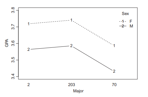
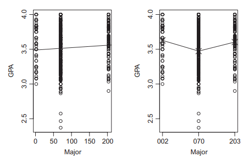
Suppose you want to predict $Y=$ GPA as a function of the two nominal variables “Major” and “Sex.” Since these are nominal variables, you should first look at the data to see how many observations there are for the different (Major, Sex) combinations, by using the “table” function table (grades\$sex, grades\$major), which gives you:
$$
\begin{array}{lrrrrrrr}
& 2 & 66 & 70 & 114 & 115 & 118 & 203 \
\text { F } & 25 & 0 & 87 & 0 & 0 & 0 & 11 \
\text { M } & 36 & 10 & 232 & 4 & 2 & 3 & 84
\end{array}
$$
The categories of the “Major” variable are coded numerically, with values 2, 66, …, 203, but there are actual degree programs attached to these numerical codes, as shown in Table 10.1 .
Notice from use of the “table” function above that there are few observations, and no females at all, in the MS programs except for the MS Accounting program. We will drop those data, but this is not an absolute requirement. Mainly, we will drop these data to make the main points more easily. Empty cells such as (Female, MS Finance) are allowed, but add a layer of complication.
So we will first subset the data as follows.
$$
\begin{aligned}
& \text { grades } 1=\text { subset (grades, major } \frac{0}{b} \text { in } \frac{\circ}{6} \mathrm{c}(2,70,203) \text { ) } \
& \text { attach (grades } 1)
\end{aligned}
$$
统计代写|回归分析代写Regression Analysis代考|Nested Model Sequence, Version 2
Model 2.0: GPA $=\beta_0+\varepsilon$
Model 2.1: GPA $=\beta_0+\beta_2$ Major.070 $+\beta_3$ Major. $203+\varepsilon$
$$
\begin{aligned}
& \text { Model 2.2: GPA }=\beta_0+\beta_1 \text { Male }+\beta_2 \text { Major.070 }+\beta_3 \text { Major.203 }+\varepsilon \
& \text { Model 2.3: GPA }=\beta_0+\beta_1 \text { Male }+\beta_2 \text { Major.070 }+\beta_3 \text { Major.203 }+\beta_4 \text { Male } \times \text { Major.070 } \
& +\beta_5 \text { Male } \times \text { Major. } 203+\varepsilon \
&
\end{aligned}
$$
The only difference between the two nested model sequences is in models 2.1 and 1.1. You might like to test models 1.1 and 2.1 in the same sequence, but you cannot because neither is a full model relative to the other. With sequences of $F$ tests, you must ensure that every model in the sequence is nested in the next one.
You can test these all simultaneously via
anova(fit2.0, fit2.1, fit2.2, fit2.3)
which yields the following output:
Analysis of Variance Table
Model 1: gpa $~ 1$
Model 2: gpa $\sim$ major
Model 3: gpa $\sim$ sex + major
Model 4: gpa $\sim$ sex + major + sex * major
Res.Df RSS Df Sum of Sq F $\operatorname{Pr}(>F)$
$1 \quad 474 \quad 42.347$
$2 \quad 47240.2892 \quad 2.05772 \quad 12.7842 \quad 3.926 \mathrm{e}-06 \quad * * *$
$344138.180 \quad 1 \quad 2.1097626 .2150 \quad 4.466 \mathrm{e}-07 \quad k \star \star$
$\begin{array}{lllllll}4 & 469 & 37.745 \quad 2 & 0.43501 & 2.7026 & 0.06807\end{array}$.
Interpretations are as follows, from bottom up:
- The interaction effects are explainable by chance alone, assuming a model where there are no interaction effects $\left(F_{2,469}=2.7026, p=0.06807\right)$.
- The effect of Sex is not easily explained by chance alone, assuming a model with only Major effects $\left(F_{1,471}=26.2150, p=4.466 \times 10^{-7}\right)$.
- The effect of Major is not easily explained by chance alone, assuming a model where nothing affects GPA $\left(F_{2,472}=12.7842, p=3.926 \times 10^{-6}\right)$.
回归分析代写
统计代写|回归分析代写Regression Analysis代考|Two Nominal Variables (Two-Way ANOVA)
再看一下平均绩点数据集:
成绩= read.table(“https://raw.githubusercontent.com/andrea2719/ . .
“URA-DataSets/master/gpa_gmat.txt”)
姓名(年级)
成绩=阅读。表$($ https://raw.githubusercontent.com/andrea2719/
“URA-DataSets/master/gpa_gmat.txt”)
姓名(年级)
这会给你:
[1]“毕业”“gpa”“gmat”“专业”“学位”“性别”“种族”
假设您希望预测$Y=$ GPA作为两个名义变量“Major”和“Sex”的函数。由于这些都是名义变量,您应该首先查看数据,通过使用“table”函数表(grades$ Sex, grades$ Major)来查看不同(Major, Sex)组合有多少观察值,它会给您:
$$
\begin{array}{lrrrrrrr}
& 2 & 66 & 70 & 114 & 115 & 118 & 203 \
\text { F } & 25 & 0 & 87 & 0 & 0 & 0 & 11 \
\text { M } & 36 & 10 & 232 & 4 & 2 & 3 & 84
\end{array}
$$
“Major”变量的类别用数字编码,值为2,66,…,203,但实际的学位课程附加在这些数字代码上,如表10.1所示。
从上面的“table”函数的使用中可以看出,除了MS会计程序外,MS程序中几乎没有观察结果,而且根本没有女性。我们将删除这些数据,但这不是绝对要求。主要是,我们将省略这些数据,使要点更容易。像(Female, MS Finance)这样的空单元格是允许的,但是增加了一层复杂性。
因此,我们将首先对数据进行如下子集处理。
$$
\begin{aligned}
& \text { grades } 1=\text { subset (grades, major } \frac{0}{b} \text { in } \frac{\circ}{6} \mathrm{c}(2,70,203) \text { ) } \
& \text { attach (grades } 1)
\end{aligned}
$$
统计代写|回归分析代写Regression Analysis代考|Nested Model Sequence, Version 2
模型2.0:GPA $=\beta_0+\varepsilon$
模型2.1:GPA $=\beta_0+\beta_2$ Major.070 $+\beta_3$ Major。 $203+\varepsilon$
$$
\begin{aligned}
& \text { Model 2.2: GPA }=\beta_0+\beta_1 \text { Male }+\beta_2 \text { Major.070 }+\beta_3 \text { Major.203 }+\varepsilon \
& \text { Model 2.3: GPA }=\beta_0+\beta_1 \text { Male }+\beta_2 \text { Major.070 }+\beta_3 \text { Major.203 }+\beta_4 \text { Male } \times \text { Major.070 } \
& +\beta_5 \text { Male } \times \text { Major. } 203+\varepsilon \
&
\end{aligned}
$$
两个嵌套模型序列之间的唯一区别在于模型2.1和1.1。您可能希望以相同的顺序测试模型1.1和2.1,但是您不能这样做,因为两者都不是一个完整的模型。对于$F$测试序列,您必须确保序列中的每个模型都嵌套在下一个模型中。
你可以同时通过
方差分析(fit2.0, fit2.1, fit2.2, fit2.3)
它产生以下输出:
方差分析表
模型1:gpa $~ 1$
模式二:gpa $\sim$ major
模式三:gpa $\sim$性别+专业
模型四:gpa $\sim$性别+专业+性别*专业
res。Df RSS Df Sq F的和$\operatorname{Pr}(>F)$
$1 \quad 474 \quad 42.347$
$2 \quad 47240.2892 \quad 2.05772 \quad 12.7842 \quad 3.926 \mathrm{e}-06 \quad * * *$
$344138.180 \quad 1 \quad 2.1097626 .2150 \quad 4.466 \mathrm{e}-07 \quad k \star \star$
$\begin{array}{lllllll}4 & 469 & 37.745 \quad 2 & 0.43501 & 2.7026 & 0.06807\end{array}$。
从下到上的解释如下:
假设一个没有相互作用的模型$\left(F_{2,469}=2.7026, p=0.06807\right)$,相互作用的影响只能通过偶然来解释。
性别的影响不容易仅仅用偶然来解释,假设一个只有主要影响的模型$\left(F_{1,471}=26.2150, p=4.466 \times 10^{-7}\right)$。
假设一个不影响GPA $\left(F_{2,472}=12.7842, p=3.926 \times 10^{-6}\right)$的模型,专业的影响不容易仅仅用偶然来解释。

统计代写|回归分析代写Regression Analysis代考 请认准UprivateTA™. UprivateTA™为您的留学生涯保驾护航。
微观经济学代写
微观经济学是主流经济学的一个分支,研究个人和企业在做出有关稀缺资源分配的决策时的行为以及这些个人和企业之间的相互作用。my-assignmentexpert™ 为您的留学生涯保驾护航 在数学Mathematics作业代写方面已经树立了自己的口碑, 保证靠谱, 高质且原创的数学Mathematics代写服务。我们的专家在图论代写Graph Theory代写方面经验极为丰富,各种图论代写Graph Theory相关的作业也就用不着 说。
线性代数代写
线性代数是数学的一个分支,涉及线性方程,如:线性图,如:以及它们在向量空间和通过矩阵的表示。线性代数是几乎所有数学领域的核心。
博弈论代写
现代博弈论始于约翰-冯-诺伊曼(John von Neumann)提出的两人零和博弈中的混合策略均衡的观点及其证明。冯-诺依曼的原始证明使用了关于连续映射到紧凑凸集的布劳威尔定点定理,这成为博弈论和数学经济学的标准方法。在他的论文之后,1944年,他与奥斯卡-莫根斯特恩(Oskar Morgenstern)共同撰写了《游戏和经济行为理论》一书,该书考虑了几个参与者的合作游戏。这本书的第二版提供了预期效用的公理理论,使数理统计学家和经济学家能够处理不确定性下的决策。
微积分代写
微积分,最初被称为无穷小微积分或 “无穷小的微积分”,是对连续变化的数学研究,就像几何学是对形状的研究,而代数是对算术运算的概括研究一样。
它有两个主要分支,微分和积分;微分涉及瞬时变化率和曲线的斜率,而积分涉及数量的累积,以及曲线下或曲线之间的面积。这两个分支通过微积分的基本定理相互联系,它们利用了无限序列和无限级数收敛到一个明确定义的极限的基本概念 。
计量经济学代写
什么是计量经济学?
计量经济学是统计学和数学模型的定量应用,使用数据来发展理论或测试经济学中的现有假设,并根据历史数据预测未来趋势。它对现实世界的数据进行统计试验,然后将结果与被测试的理论进行比较和对比。
根据你是对测试现有理论感兴趣,还是对利用现有数据在这些观察的基础上提出新的假设感兴趣,计量经济学可以细分为两大类:理论和应用。那些经常从事这种实践的人通常被称为计量经济学家。
Matlab代写
MATLAB 是一种用于技术计算的高性能语言。它将计算、可视化和编程集成在一个易于使用的环境中,其中问题和解决方案以熟悉的数学符号表示。典型用途包括:数学和计算算法开发建模、仿真和原型制作数据分析、探索和可视化科学和工程图形应用程序开发,包括图形用户界面构建MATLAB 是一个交互式系统,其基本数据元素是一个不需要维度的数组。这使您可以解决许多技术计算问题,尤其是那些具有矩阵和向量公式的问题,而只需用 C 或 Fortran 等标量非交互式语言编写程序所需的时间的一小部分。MATLAB 名称代表矩阵实验室。MATLAB 最初的编写目的是提供对由 LINPACK 和 EISPACK 项目开发的矩阵软件的轻松访问,这两个项目共同代表了矩阵计算软件的最新技术。MATLAB 经过多年的发展,得到了许多用户的投入。在大学环境中,它是数学、工程和科学入门和高级课程的标准教学工具。在工业领域,MATLAB 是高效研究、开发和分析的首选工具。MATLAB 具有一系列称为工具箱的特定于应用程序的解决方案。对于大多数 MATLAB 用户来说非常重要,工具箱允许您学习和应用专业技术。工具箱是 MATLAB 函数(M 文件)的综合集合,可扩展 MATLAB 环境以解决特定类别的问题。可用工具箱的领域包括信号处理、控制系统、神经网络、模糊逻辑、小波、仿真等。