如果你也在 怎样代写回归分析Regression Analysis 这个学科遇到相关的难题,请随时右上角联系我们的24/7代写客服。回归分析Regression Analysis被广泛用于预测和预报,其使用与机器学习领域有很大的重叠。在某些情况下,回归分析可以用来推断自变量和因变量之间的因果关系。重要的是,回归本身只揭示了固定数据集中因变量和自变量集合之间的关系。为了分别使用回归进行预测或推断因果关系,研究者必须仔细论证为什么现有的关系对新的环境具有预测能力,或者为什么两个变量之间的关系具有因果解释。当研究者希望使用观察数据来估计因果关系时,后者尤其重要。
回归分析Regression Analysis在统计建模中,回归分析是一组统计过程,用于估计因变量(通常称为 “结果 “或 “响应 “变量,或机器学习术语中的 “标签”)与一个或多个自变量(通常称为 “预测因子”、”协变量”、”解释变量 “或 “特征”)之间的关系。回归分析最常见的形式是线性回归,即根据特定的数学标准找到最适合数据的直线(或更复杂的线性组合)。例如,普通最小二乘法计算唯一的直线(或超平面),使真实数据与该直线(或超平面)之间的平方差之和最小。由于特定的数学原因(见线性回归),这使得研究者能够在自变量具有一组给定值时估计因变量的条件期望值(或人口平均值)。不太常见的回归形式使用稍微不同的程序来估计替代位置参数(例如,量化回归或必要条件分析),或在更广泛的非线性模型集合中估计条件期望值(例如,非参数回归)。
回归分析Regression Analysis代写,免费提交作业要求, 满意后付款,成绩80\%以下全额退款,安全省心无顾虑。专业硕 博写手团队,所有订单可靠准时,保证 100% 原创。 最高质量的回归分析Regression Analysis作业代写,服务覆盖北美、欧洲、澳洲等 国家。 在代写价格方面,考虑到同学们的经济条件,在保障代写质量的前提下,我们为客户提供最合理的价格。 由于作业种类很多,同时其中的大部分作业在字数上都没有具体要求,因此回归分析Regression Analysis作业代写的价格不固定。通常在专家查看完作业要求之后会给出报价。作业难度和截止日期对价格也有很大的影响。
同学们在留学期间,都对各式各样的作业考试很是头疼,如果你无从下手,不如考虑my-assignmentexpert™!
my-assignmentexpert™提供最专业的一站式服务:Essay代写,Dissertation代写,Assignment代写,Paper代写,Proposal代写,Proposal代写,Literature Review代写,Online Course,Exam代考等等。my-assignmentexpert™专注为留学生提供Essay代写服务,拥有各个专业的博硕教师团队帮您代写,免费修改及辅导,保证成果完成的效率和质量。同时有多家检测平台帐号,包括Turnitin高级账户,检测论文不会留痕,写好后检测修改,放心可靠,经得起任何考验!
想知道您作业确定的价格吗? 免费下单以相关学科的专家能了解具体的要求之后在1-3个小时就提出价格。专家的 报价比上列的价格能便宜好几倍。
我们在统计Statistics代写方面已经树立了自己的口碑, 保证靠谱, 高质且原创的统计Statistics代写服务。我们的专家在回归分析Regression Analysis代写方面经验极为丰富,各种回归分析Regression Analysis相关的作业也就用不着 说。

统计代写|回归分析代写Regression Analysis代考|Testing for Heteroscedasticity Using the Production Cost Data
The method is fairly simple as the following code shows.
ProdC = read.table(“https://raw.githubusercontent.com/andrea2719/
URA-DataSets/master/ProdC.txt”)
fit $=1 \mathrm{~m}($ Cost $\sim$ Widgets, data=ProdC)
y.hat $=$ fit\$fitted.values; resid = fit\$residuals; abs.resid = abs(resid)
fit.glejser $=1 \mathrm{~m}(a b s . r e s i d \sim y \cdot h a t)$
summary(fit.glejser)
Prodc $=$ read.table $($ “https: $/ /$ raw.githubusercontent.com/andrea $2719 /$
URA-Datasets/master/ProdC.txt”)
fit $=\operatorname{lm}$ (Cost $\sim$ Widgets, data=ProdC)
$y \cdot h a t=$ fit\$fitted.values; resid $=$ fit\$residuals; abs.resid = abs(resid)
fit.glejser $=1 \mathrm{~m}(a b s . r e s i d \sim y \cdot$ hat $)$
summary(fit.glejser)
The relevant output is as follows:
Coefficients:
$\begin{array}{lrrrr} & \text { Estimate } & \text { Std. Error } t \text { value } \operatorname{Pr}(>|t|) \ \text { (Intercept) } & 1.800 \mathrm{e}+02 & 9.464 \mathrm{e}+01 & 1.902 & 0.0648 \ \text { y.hat } & 7.196 \mathrm{e}-03 & 4.491 \mathrm{e}-02 & 0.160 & 0.8736\end{array}$
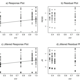
This output is related to the right panel of Figure 4.6. The positive coefficient $7.196 \mathrm{e}-03$ of y. hat suggests that, if there is a linear trend in the graph, it is upward. However, such an upward trend is explainable by chance alone $(p=0.8736)$, so, again, there is no compelling evidence of heteroscedasticity in the process that produced these data.
But the test does not prove homoscedasticity. You know, a priori, that it is impossible for the conditional distributions of Cost to all have precisely the same variances, to the infinite decimal. Further, for jobs with more Widgets, there is simply more room for variability in Cost (since the Cost values are farther from 0); thus, subject matter considerations suggest that variability in Cost indeed does increase for jobs where number of Widgets is larger. But such heteroscedasticity was not proven using the data, because the positive trend in Cost variance for larger Widgets is explainable by chance alone.
统计代写|回归分析代写Regression Analysis代考|Testing for Heteroscedasticity Using the Personal Assets Data
The code looks just like the code used for the Production Cost analysis.
Pass $=$ read.table(“https://raw.githubusercontent.com/andrea2719/
URA-DataSets/master/Pass.txt”)
attach(Pass) ; fit $=1 \mathrm{~m}($ P.assets $\sim$ Age)
y.hat $=$ fit\$fitted.values; resid = fit\$residuals; abs.resid = abs(resid)
fit.glejser $=1 \mathrm{~m}(a b s . r e s i d ~ y . h a t)$
summary(fit.glejser)
Pass $=$ read.table $($ “https: $/ /$ raw.githubusercontent. com/andrea2719/
URA-Datasets/master/Pass.txt”)
attach (Pass) ; fit $=1 \mathrm{~m}($ P. assets $\sim$ Age)
$y \cdot$ hat $=$ fit\$fitted.values; resid = fit\$residuals; abs.resid $=$ abs (resid)
fit.glejser $=\operatorname{lm}(a b s \cdot r e s i d \sim y \cdot h a t)$
summary (fit.glejser)
The relevant output is as follows:
Coefficients:
This output is related to the right panel of Figure 4.7. The positive coefficient 0.18500 of y.hat suggests what you can plainly see; namely, that there is an upward trend in that graph. Such an upward trend is not easily explained by chance alone $(p=0.000877)$.
As always, the results should make sense from a subject matter standpoint. Here, the increase in variability is expected, because as people get older, they generally have more money and have had more time to accrue personal assets. But most importantly, this ability to accrue more, coupled with people’s personal choice as to whether they wish to accrue more, is what causes increased variability in personal assets with increasing age. People may have much money but simply choose to live more simply, and have few personal assets. Others with the same amount of money choose to accrue many items, leading to a large range of variability in the high-income group. On the other hand, people with little money have less choice as to whether they may accrue many or few assets, leading to smaller variability in that group. Thus, choice and opportunity cause the heteroscedasticity that is apparent in the data of this example.
回归分析代写
统计代写|回归分析代写Regression Analysis代考|Testing for Heteroscedasticity Using the Production Cost Data
方法非常简单,如下面的代码所示。
ProdC = read.table(“https://raw.githubusercontent.com/andrea2719/
URA-DataSets/master/ proc .txt”)
fit $=1 \mathrm{~m}($ Cost $\sim$ Widgets, data=ProdC)
y。帽子$=$ fit$ fits .values;ressid = fit$residuals;abs.resid = abs(resid)
fit。glejser $=1 \mathrm{~m}(a b s . r e s i d \sim y \cdot h a t)$
summary(fit.glejser)
Prodc $=$ read。表$($ “https: $/ /$ raw.githubusercontent.com/andrea $2719 /$
URA-Datasets/master/ product .txt”)
fit $=\operatorname{lm}$ (Cost $\sim$ Widgets, data=ProdC)
$y \cdot h a t=$ fit$ fits .values;Resid $=$ fit$残差;abs.resid = abs(resid)
fit。glejser $=1 \mathrm{~m}(a b s . r e s i d \sim y \cdot$ hat $)$
summary(fit.glejser)
相关输出如下:
Coefficients:
$\begin{array}{lrrrr} & \text { Estimate } & \text { Std. Error } t \text { value } \operatorname{Pr}(>|t|) \ \text { (Intercept) } & 1.800 \mathrm{e}+02 & 9.464 \mathrm{e}+01 & 1.902 & 0.0648 \ \text { y.hat } & 7.196 \mathrm{e}-03 & 4.491 \mathrm{e}-02 & 0.160 & 0.8736\end{array}$
此输出与图4.6右侧面板相关。y. hat的正系数$7.196 \mathrm{e}-03$表明,如果在图中存在线性趋势,则是向上的。然而,这种上升趋势只能通过偶然的机会来解释$(p=0.8736)$,因此,在产生这些数据的过程中,再一次没有令人信服的异方差证据。
但该检验不能证明异方差性。你知道,先验地,Cost的条件分布不可能都有完全相同的方差,直到无穷大的小数。此外,对于具有更多小部件的作业,成本的变化空间更大(因为成本值离0更远);因此,主题方面的考虑表明,对于widget数量较多的作业,成本的可变性确实会增加。但是,这种异方差并没有使用数据来证明,因为较大部件的成本方差的正趋势只能用偶然来解释。
统计代写|回归分析代写Regression Analysis代考|Testing for Heteroscedasticity Using the Personal Assets Data
代码看起来就像用于生产成本分析的代码。
Pass $=$ read.table(“https://raw.githubusercontent.com/andrea2719/
URA-DataSets/master/Pass.txt”)
attach(Pass);fit $=1 \mathrm{~m}($ P.assets $\sim$年龄)
y。帽子$=$ fit$ fits .values;ressid = fit$residuals;abs.resid = abs(resid)
fit。glejser $=1 \mathrm{~m}(a b s . r e s i d ~ y . h a t)$
summary(fit.glejser)
Pass $=$ read。表$($ “https: $/ /$ raw.githubusercontent。
data /master/Pass.txt
attach (Pass);fit $=1 \mathrm{~m}($ P. assets $\sim$ Age)
$y \cdot$ hat $=$ fit$ fits .values;ressid = fit$residuals;abs.resid $=$ abs (resid)
fit。glejser $=\operatorname{lm}(a b s \cdot r e s i d \sim y \cdot h a t)$
summary (fit.glejser)
相关输出如下:
Coefficients:
此输出与图4.7右侧面板相关。y的正系数0.18500表明你可以清楚地看到;也就是说,图表上有一个上升的趋势。这种上升趋势不容易仅仅用偶然来解释$(p=0.000877)$ .
一如既往,从主题的角度来看,结果应该是有意义的。在这里,可变性的增加是意料之中的,因为随着人们年龄的增长,他们通常有更多的钱,有更多的时间积累个人资产。但最重要的是,这种积累更多财富的能力,加上人们是否希望积累更多财富的个人选择,是导致个人资产随着年龄增长而变化的原因。人们可能有很多钱,但只是选择更简单的生活,很少有个人资产。其他拥有同样多钱的人选择累积很多项目,导致高收入群体的差异很大。另一方面,没有钱的人在积累更多或更少资产方面的选择更少,导致这一群体的可变性更小。因此,选择和机会导致了本例数据中明显的异方差。

统计代写|回归分析代写Regression Analysis代考 请认准UprivateTA™. UprivateTA™为您的留学生涯保驾护航。
微观经济学代写
微观经济学是主流经济学的一个分支,研究个人和企业在做出有关稀缺资源分配的决策时的行为以及这些个人和企业之间的相互作用。my-assignmentexpert™ 为您的留学生涯保驾护航 在数学Mathematics作业代写方面已经树立了自己的口碑, 保证靠谱, 高质且原创的数学Mathematics代写服务。我们的专家在图论代写Graph Theory代写方面经验极为丰富,各种图论代写Graph Theory相关的作业也就用不着 说。
线性代数代写
线性代数是数学的一个分支,涉及线性方程,如:线性图,如:以及它们在向量空间和通过矩阵的表示。线性代数是几乎所有数学领域的核心。
博弈论代写
现代博弈论始于约翰-冯-诺伊曼(John von Neumann)提出的两人零和博弈中的混合策略均衡的观点及其证明。冯-诺依曼的原始证明使用了关于连续映射到紧凑凸集的布劳威尔定点定理,这成为博弈论和数学经济学的标准方法。在他的论文之后,1944年,他与奥斯卡-莫根斯特恩(Oskar Morgenstern)共同撰写了《游戏和经济行为理论》一书,该书考虑了几个参与者的合作游戏。这本书的第二版提供了预期效用的公理理论,使数理统计学家和经济学家能够处理不确定性下的决策。
微积分代写
微积分,最初被称为无穷小微积分或 “无穷小的微积分”,是对连续变化的数学研究,就像几何学是对形状的研究,而代数是对算术运算的概括研究一样。
它有两个主要分支,微分和积分;微分涉及瞬时变化率和曲线的斜率,而积分涉及数量的累积,以及曲线下或曲线之间的面积。这两个分支通过微积分的基本定理相互联系,它们利用了无限序列和无限级数收敛到一个明确定义的极限的基本概念 。
计量经济学代写
什么是计量经济学?
计量经济学是统计学和数学模型的定量应用,使用数据来发展理论或测试经济学中的现有假设,并根据历史数据预测未来趋势。它对现实世界的数据进行统计试验,然后将结果与被测试的理论进行比较和对比。
根据你是对测试现有理论感兴趣,还是对利用现有数据在这些观察的基础上提出新的假设感兴趣,计量经济学可以细分为两大类:理论和应用。那些经常从事这种实践的人通常被称为计量经济学家。
Matlab代写
MATLAB 是一种用于技术计算的高性能语言。它将计算、可视化和编程集成在一个易于使用的环境中,其中问题和解决方案以熟悉的数学符号表示。典型用途包括:数学和计算算法开发建模、仿真和原型制作数据分析、探索和可视化科学和工程图形应用程序开发,包括图形用户界面构建MATLAB 是一个交互式系统,其基本数据元素是一个不需要维度的数组。这使您可以解决许多技术计算问题,尤其是那些具有矩阵和向量公式的问题,而只需用 C 或 Fortran 等标量非交互式语言编写程序所需的时间的一小部分。MATLAB 名称代表矩阵实验室。MATLAB 最初的编写目的是提供对由 LINPACK 和 EISPACK 项目开发的矩阵软件的轻松访问,这两个项目共同代表了矩阵计算软件的最新技术。MATLAB 经过多年的发展,得到了许多用户的投入。在大学环境中,它是数学、工程和科学入门和高级课程的标准教学工具。在工业领域,MATLAB 是高效研究、开发和分析的首选工具。MATLAB 具有一系列称为工具箱的特定于应用程序的解决方案。对于大多数 MATLAB 用户来说非常重要,工具箱允许您学习和应用专业技术。工具箱是 MATLAB 函数(M 文件)的综合集合,可扩展 MATLAB 环境以解决特定类别的问题。可用工具箱的领域包括信号处理、控制系统、神经网络、模糊逻辑、小波、仿真等。