如果你也在 怎样代写线性回归Linear Regression 这个学科遇到相关的难题,请随时右上角联系我们的24/7代写客服。线性回归Linear Regression在统计学中,是对标量响应和一个或多个解释变量(也称为因变量和自变量)之间的关系进行建模的一种线性方法。一个解释变量的情况被称为简单线性回归;对于一个以上的解释变量,这一过程被称为多元线性回归。这一术语不同于多元线性回归,在多元线性回归中,预测的是多个相关的因变量,而不是一个标量变量。
线性回归Linear Regression在线性回归中,关系是用线性预测函数建模的,其未知的模型参数是根据数据估计的。最常见的是,假设给定解释变量(或预测因子)值的响应的条件平均值是这些值的仿生函数;不太常见的是,使用条件中位数或其他一些量化指标。像所有形式的回归分析一样,线性回归关注的是给定预测因子值的反应的条件概率分布,而不是所有这些变量的联合概率分布,这是多元分析的领域。
线性回归Linear Regression代写,免费提交作业要求, 满意后付款,成绩80\%以下全额退款,安全省心无顾虑。专业硕 博写手团队,所有订单可靠准时,保证 100% 原创。最高质量的线性回归Linear Regression作业代写,服务覆盖北美、欧洲、澳洲等 国家。 在代写价格方面,考虑到同学们的经济条件,在保障代写质量的前提下,我们为客户提供最合理的价格。 由于作业种类很多,同时其中的大部分作业在字数上都没有具体要求,因此线性回归Linear Regression作业代写的价格不固定。通常在专家查看完作业要求之后会给出报价。作业难度和截止日期对价格也有很大的影响。
同学们在留学期间,都对各式各样的作业考试很是头疼,如果你无从下手,不如考虑my-assignmentexpert™!
my-assignmentexpert™提供最专业的一站式服务:Essay代写,Dissertation代写,Assignment代写,Paper代写,Proposal代写,Proposal代写,Literature Review代写,Online Course,Exam代考等等。my-assignmentexpert™专注为留学生提供Essay代写服务,拥有各个专业的博硕教师团队帮您代写,免费修改及辅导,保证成果完成的效率和质量。同时有多家检测平台帐号,包括Turnitin高级账户,检测论文不会留痕,写好后检测修改,放心可靠,经得起任何考验!
想知道您作业确定的价格吗? 免费下单以相关学科的专家能了解具体的要求之后在1-3个小时就提出价格。专家的 报价比上列的价格能便宜好几倍。
我们在统计Statistics代写方面已经树立了自己的口碑, 保证靠谱, 高质且原创的统计Statistics代写服务。我们的专家在线性回归Linear Regression代写方面经验极为丰富,各种线性回归Linear Regression相关的作业也就用不着说。
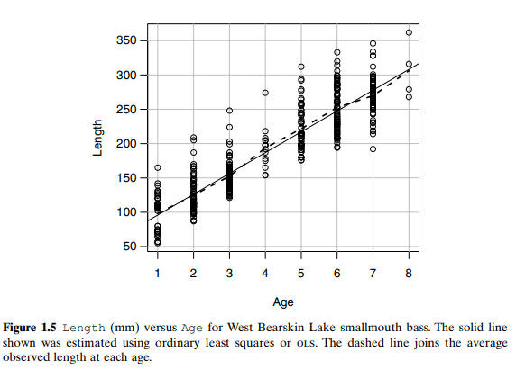
统计代写|线性回归代写Linear Regression代考|ADDING A TERM TO A SIMPLE LINEAR REGRESSION MODEL
We start with a response $Y$ and the simple linear regression mean function
$$
\mathrm{E}\left(Y \mid X_1=x_1\right)=\beta_0+\beta_1 x_1
$$
Now suppose we have a second variable $X_2$ with which to predict the response. By adding $X_2$ to the problem, we will get a mean function that depends on both the value of $X_1$ and the value of $X_2$,
$$
\mathrm{E}\left(Y \mid X_1=x_1, X_2=x_2\right)=\beta_0+\beta_1 x_1+\beta_2 x_2
$$
The main idea in adding $X_2$ is to explain the part of $Y$ that has not already been explained by $X_1$.
United Nations Data
We will reconsider the United Nations data discussed in Problem 1.3. To the regression of $\log$ (Fertility), the base-two $\log$ fertility rate on $\log (P P g d p)$, the base-two $\log$ of the per person gross domestic product, we consider adding Purban, the percentage of the population that lives in an urban area. The data in the file UN2 . txt give values for these three variables, as well as the name of the Locality for 193 localities, mostly countries, for which the United Nations provides data.
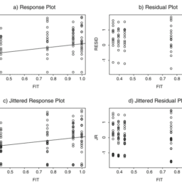
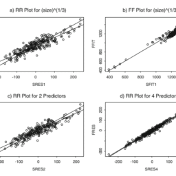
Figure 3.1 presents several graphical views of these data. Figure 3.1a can be viewed as a summary graph for the simple regression of $\log$ (Fertility) on $\log (P P g d p)$. The fitted mean function using oLS is
$$
\widehat{\mathrm{E}}(\log (\text { Fertility }) \mid \log (P P g d p))=2.703-0.153 \log (\text { PPgdp })
$$
with $R^2=0.459$, so about $46 \%$ of the variability in $\log$ (Fertility) is explained by $\log (P P g d p)$. An increase of one unit in $\log (P P g d p)$, which corresponds to a doubling of $P P g d p$, is estimated to decrease $\log$ (Fertility) by 0.153 units.
Similarly, Figure $3.1 \mathrm{~b}$ is the summary graph for the regression of $\log$ (Fertility) on Purban. This simple regression has fitted mean function
$$
\widehat{\mathrm{E}}(\log (\text { Fertility }) \mid \text { Purban })=1.750-0.013 \text { Purban }
$$
with $R^2=0.348$, so Purban explains about $35 \%$ of the variability in $\log$ (Fertility).
统计代写|线性回归代写Linear Regression代考|Explaining Variability
Given these graphs, what can be said about the proportion of variability in $\log ($ Fertility) explained by $\log (P P g d p)$ and Purban? We can say that the total explained variation must exceed 46 percent, the larger of the two values explained by each variable separately, since using both $\log (P P g d p)$ and Purban must surely be at least as informative as using just one of them. The total variation will be additive, $46 \%+35 \%=91 \%$, only if the two variables are completely unrelated and measure different things. The total can be less than the sum if the terms are related and are at least in part explaining the same variation. Finally, the total can exceed the sum if the two variables act jointly so that knowing both gives more information than knowing just one of them. For example, the area of a rectangle may be only poorly determined by either the length or width alone, but if both are considered at the same time, area can be determined exactly. It is precisely this inability to predict the joint relationship from the marginal relationships that makes multiple regression rich and complicated.
Added-Variable Plots
The unique effect of adding Purban to a mean function that already includes $\log (P P g d p)$ is determined by the relationship between the part of $\log$ (Fertility) that is not explained by $\log (P P g d p)$ and the part of Purban that is not explained by $\log (P P g d p)$. The “unexplained parts” are just the residuals from these two simple regressions, and so we need to examine the scatterplot of the residuals from the regression of $\log$ (Fertility) on $\log (P P g d p)$ versus the residuals from the regression of Purban on $\log (P P g d p)$. This plot is shown in Figure 3.1d. Figure 3.1b is the summary graph for the relationship between $\log$ (Fertility) and Purban ignoring $\log (P P g d p)$, while Figure 3.1d shows this relationship, but after adjusting for $\log (P P g d p)$. If Figure 3.1d shows a stronger relationship than does Figure 3.1b, meaning that the points in the plot show less variation about the fitted straight line,then the two variables act jointly to explain extra variation, while if the relationship is weaker, or the plot exhibits more variation, then the total explained variability is less than the additive amount. The latter seems to be the case here.
If we fit the simple regression mean function to Figure $3.1 \mathrm{~d}$, the fitted line has zero intercept, since the averages of the two plotted variables are zero, and the estimated slope via oLS is $\hat{\beta}_2=-0.0035 \approx-0.004$. It turns out that this is exactly the estimate $\hat{\beta}_2$ that would be obtained using oLs to get the estimates using the mean function (3.1). Figure $3.1 \mathrm{~d}$ is called an added-variable plot.
线性回归代写
统计代写|线性回归代写Linear Regression代考|ADDING A TERM TO A SIMPLE LINEAR REGRESSION MODEL
我们从响应$Y$和简单的线性回归均值函数开始
$$
\mathrm{E}\left(Y \mid X_1=x_1\right)=\beta_0+\beta_1 x_1
$$
现在假设我们有第二个变量$X_2$来预测响应。通过将$X_2$添加到问题中,我们将得到一个同时依赖于$X_1$和$X_2$值的均值函数,
$$
\mathrm{E}\left(Y \mid X_1=x_1, X_2=x_2\right)=\beta_0+\beta_1 x_1+\beta_2 x_2
$$
添加$X_2$的主要目的是解释$Y$中尚未被$X_1$解释的部分。
联合国数据
我们将重新考虑问题1.3中讨论的联合国数据。对于回归$\log$(生育率),$\log (P P g d p)$上的基数2 $\log$生育率,人均国内生产总值的基数2 $\log$,我们考虑加入Purban,即居住在城市地区的人口比例。UN2文件中的数据。txt给出了这三个变量的值,以及193个地点(主要是联合国提供数据的国家)的地点名称。
图3.1展示了这些数据的几个图形视图。图3.1a可以看作是$\log (P P g d p)$上$\log$(生育率)简单回归的汇总图。使用oLS拟合的均值函数为
$$
\widehat{\mathrm{E}}(\log (\text { Fertility }) \mid \log (P P g d p))=2.703-0.153 \log (\text { PPgdp })
$$
与$R^2=0.459$,所以关于$46 \%$的变异在$\log$(生育率)是由$\log (P P g d p)$解释。据估计,$\log (P P g d p)$每增加1个单位,相当于$P P g d p$增加一倍,$\log$(生育率)就会减少0.153个单位。
同样,图$3.1 \mathrm{~b}$是$\log$(生育率)对城市人口回归的汇总图。这个简单的回归具有拟合的均值函数
$$
\widehat{\mathrm{E}}(\log (\text { Fertility }) \mid \text { Purban })=1.750-0.013 \text { Purban }
$$
与$R^2=0.348$,所以Purban解释了$\log$(生育率)的变异$35 \%$。
统计代写|线性回归代写Linear Regression代考|Explaining Variability
鉴于这些图表,$\log (P P g d p)$和Purban解释的$\log ($ Fertility)的变异性比例有什么可说的?我们可以说,总解释的变化必须超过46%,即每个变量单独解释的两个值中较大的那个,因为同时使用$\log (P P g d p)$和Purban肯定至少与只使用其中一个一样具有信息量。只有当两个变量完全不相关并且测量不同的东西时,总变化才会是相加的,$46 \%+35 \%=91 \%$。如果这些术语是相关的,并且至少部分地解释了相同的变化,则总数可以小于总和。最后,如果两个变量共同作用,那么知道两个变量提供的信息比只知道其中一个变量提供的信息更多,那么总数可能会超过总和。例如,矩形的面积可能仅由长度或宽度来确定,但如果同时考虑两者,则可以精确地确定面积。正是由于不能从边际关系中预测联合关系,使得多元回归丰富而复杂。
附加变量图
将Purban添加到已经包含$\log (P P g d p)$的平均函数中的独特效果是由$\log$(生育率)中未被$\log (P P g d p)$解释的部分与未被$\log (P P g d p)$解释的部分之间的关系决定的。“无法解释的部分”只是这两个简单回归的残差,因此我们需要检查$\log$ (Fertility)在$\log (P P g d p)$上的回归与Purban在$\log (P P g d p)$上的回归的残差的散点图。该图如图3.1d所示。图3.1b是忽略$\log (P P g d p)$的$\log$ (Fertility)和Purban之间关系的汇总图,图3.1d是在调整$\log (P P g d p)$之后的关系。如果图3.1d比图3.1b的关系更强,即图中点对拟合直线的变化较小,则两个变量共同作用来解释额外的变化,而如果关系较弱,或图中表现出更多的变化,则总解释变率小于相加量。这里的情况似乎是后者。
如果我们将简单回归均值函数拟合到图$3.1 \mathrm{~d}$,则拟合线的截距为零,因为两个绘制变量的平均值为零,通过oLS估计的斜率为$\hat{\beta}_2=-0.0035 \approx-0.004$。事实证明,这正是使用oLs获得使用均值函数(3.1)的估计值$\hat{\beta}_2$。图$3.1 \mathrm{~d}$称为加变量图。

统计代写|线性回归代写Linear Regression代考 请认准UprivateTA™. UprivateTA™为您的留学生涯保驾护航。
微观经济学代写
微观经济学是主流经济学的一个分支,研究个人和企业在做出有关稀缺资源分配的决策时的行为以及这些个人和企业之间的相互作用。my-assignmentexpert™ 为您的留学生涯保驾护航 在数学Mathematics作业代写方面已经树立了自己的口碑, 保证靠谱, 高质且原创的数学Mathematics代写服务。我们的专家在图论代写Graph Theory代写方面经验极为丰富,各种图论代写Graph Theory相关的作业也就用不着 说。
线性代数代写
线性代数是数学的一个分支,涉及线性方程,如:线性图,如:以及它们在向量空间和通过矩阵的表示。线性代数是几乎所有数学领域的核心。
博弈论代写
现代博弈论始于约翰-冯-诺伊曼(John von Neumann)提出的两人零和博弈中的混合策略均衡的观点及其证明。冯-诺依曼的原始证明使用了关于连续映射到紧凑凸集的布劳威尔定点定理,这成为博弈论和数学经济学的标准方法。在他的论文之后,1944年,他与奥斯卡-莫根斯特恩(Oskar Morgenstern)共同撰写了《游戏和经济行为理论》一书,该书考虑了几个参与者的合作游戏。这本书的第二版提供了预期效用的公理理论,使数理统计学家和经济学家能够处理不确定性下的决策。
微积分代写
微积分,最初被称为无穷小微积分或 “无穷小的微积分”,是对连续变化的数学研究,就像几何学是对形状的研究,而代数是对算术运算的概括研究一样。
它有两个主要分支,微分和积分;微分涉及瞬时变化率和曲线的斜率,而积分涉及数量的累积,以及曲线下或曲线之间的面积。这两个分支通过微积分的基本定理相互联系,它们利用了无限序列和无限级数收敛到一个明确定义的极限的基本概念 。
计量经济学代写
什么是计量经济学?
计量经济学是统计学和数学模型的定量应用,使用数据来发展理论或测试经济学中的现有假设,并根据历史数据预测未来趋势。它对现实世界的数据进行统计试验,然后将结果与被测试的理论进行比较和对比。
根据你是对测试现有理论感兴趣,还是对利用现有数据在这些观察的基础上提出新的假设感兴趣,计量经济学可以细分为两大类:理论和应用。那些经常从事这种实践的人通常被称为计量经济学家。
Matlab代写
MATLAB 是一种用于技术计算的高性能语言。它将计算、可视化和编程集成在一个易于使用的环境中,其中问题和解决方案以熟悉的数学符号表示。典型用途包括:数学和计算算法开发建模、仿真和原型制作数据分析、探索和可视化科学和工程图形应用程序开发,包括图形用户界面构建MATLAB 是一个交互式系统,其基本数据元素是一个不需要维度的数组。这使您可以解决许多技术计算问题,尤其是那些具有矩阵和向量公式的问题,而只需用 C 或 Fortran 等标量非交互式语言编写程序所需的时间的一小部分。MATLAB 名称代表矩阵实验室。MATLAB 最初的编写目的是提供对由 LINPACK 和 EISPACK 项目开发的矩阵软件的轻松访问,这两个项目共同代表了矩阵计算软件的最新技术。MATLAB 经过多年的发展,得到了许多用户的投入。在大学环境中,它是数学、工程和科学入门和高级课程的标准教学工具。在工业领域,MATLAB 是高效研究、开发和分析的首选工具。MATLAB 具有一系列称为工具箱的特定于应用程序的解决方案。对于大多数 MATLAB 用户来说非常重要,工具箱允许您学习和应用专业技术。工具箱是 MATLAB 函数(M 文件)的综合集合,可扩展 MATLAB 环境以解决特定类别的问题。可用工具箱的领域包括信号处理、控制系统、神经网络、模糊逻辑、小波、仿真等。