如果你也在 怎样代写回归分析Regression Analysis 这个学科遇到相关的难题,请随时右上角联系我们的24/7代写客服。回归分析Regression Analysis回归中的概率观点具体体现在给定X数据的特定固定值的Y数据的可变性模型中。这种可变性是用条件分布建模的;因此,副标题是:“条件分布方法”。回归的整个主题都是用条件分布来表达的;这种观点统一了不同的方法,如经典回归、方差分析、泊松回归、逻辑回归、异方差回归、分位数回归、名义Y数据模型、因果模型、神经网络回归和树回归。所有这些都可以方便地用给定特定X值的Y条件分布模型来看待。
回归分析Regression Analysis条件分布是回归数据的正确模型。它们告诉你,对于变量X的给定值,可能存在可观察到的变量Y的分布。如果你碰巧知道这个分布,那么你就知道了你可能知道的关于响应变量Y的所有信息,因为它与预测变量X的给定值有关。与基于R^2统计量的典型回归方法不同,该模型解释了100%的潜在可观察到的Y数据,后者只解释了Y数据的一小部分,而且在假设几乎总是被违反的情况下也是不正确的。
回归分析Regression Analysis代写,免费提交作业要求, 满意后付款,成绩80\%以下全额退款,安全省心无顾虑。专业硕 博写手团队,所有订单可靠准时,保证 100% 原创。 最高质量的回归分析Regression Analysis作业代写,服务覆盖北美、欧洲、澳洲等 国家。 在代写价格方面,考虑到同学们的经济条件,在保障代写质量的前提下,我们为客户提供最合理的价格。 由于作业种类很多,同时其中的大部分作业在字数上都没有具体要求,因此回归分析Regression Analysis作业代写的价格不固定。通常在专家查看完作业要求之后会给出报价。作业难度和截止日期对价格也有很大的影响。
同学们在留学期间,都对各式各样的作业考试很是头疼,如果你无从下手,不如考虑my-assignmentexpert™!
my-assignmentexpert™提供最专业的一站式服务:Essay代写,Dissertation代写,Assignment代写,Paper代写,Proposal代写,Proposal代写,Literature Review代写,Online Course,Exam代考等等。my-assignmentexpert™专注为留学生提供Essay代写服务,拥有各个专业的博硕教师团队帮您代写,免费修改及辅导,保证成果完成的效率和质量。同时有多家检测平台帐号,包括Turnitin高级账户,检测论文不会留痕,写好后检测修改,放心可靠,经得起任何考验!
统计代写|回归分析代写Regression Analysis代考|Does Eating Ice Cream Cause You to Drown?
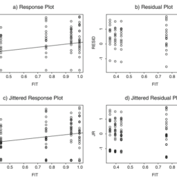
Consider the (standard) example where the response variable is $Y=$ Drowning Deaths in a week in the U.S.A., and $X=$ Ice Cream Sales that same week. There is an association between $Y$ and $X$. A scatterplot of such data might look as shown in Figure 6.2.
From the data shown in Figure 6.2, there is clearly a predictive relationship: When Ice Cream Sales are higher, the distribution of Drownings is shifted toward higher numbers. Thus, you can use $X=$ Ice Cream Sales to obtain improved predictions of $Y=$ Drownings.
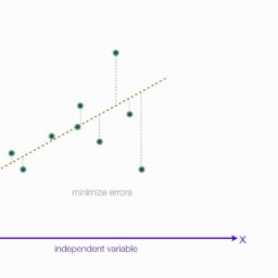
Putting a little more structure into the model, suppose the linearity assumption is met so that the means of the distributions $p(y \mid x)$ fall on a straight line, and write the following predictive model:
$$
Y=\beta_0+\beta_1 X+\varepsilon
$$
where $Y$ = Drownings, and $X=$ Ice Cream Sales. Using this model, you can logically conclude the following:
Predictive association interpretation
Consider two large sets of potentially observable weeks, one where Ice Cream Sales is equal to 250 and the other where Ice Cream Sales is equal to 350 . Then the mean of the Drownings variable is $100 \beta_1$ more in the second scenario than in the first.
The predictive association interpretation differs from the causal interpretation. The following interpretation uses a correct definition of causality, but causality does not logically follow from the predictive model.
统计代写|回归分析代写Regression Analysis代考|The Classical Multiple Regression Model and Interpretation of Its Parameters
Similar to the simple regression model, the classical multiple regression model specifies the conditional distributions that produce all observations $Y_i, i=1,2, \ldots, n$, in the data set, as well as infinitely many potentially observable observations not in the data set. But with multiple regression, these conditional distributions refer to combinations of the multiple $X$ variables.
The classical multiple regression model is given as follows:
The classical multiple regression model
$$
Y_i \mid X_{i 1}=x_{i 1}, X_{i 2}=x_{i 2}, \ldots, X_{i k}=x_{i k} \sim_{\text {ind }} \mathrm{N}\left(\beta_0+\beta_1 x_{i 1}+\beta_2 x_{i 2}+\ldots+\beta_k x_{i k}, \sigma^2\right)
$$
The case where $k=2$ is instructive. Whereas in simple linear regression (where $k=1$ ) the conditional mean function is a line that can be shown in a 2-dimensional graph, the multiple regression case where $k=2$ gives a conditional mean function that is a plane that can be shown in a 3-dimensional graph. In Figure 6.3, each point of the plane corresponds to the mean of the distribution of $Y$ for a given combination $X_1=x_1, X_2=x_2$. The following $\mathrm{R}$ code and resulting 3-D graph show this function.
R code for Figure 6.3
$\mathrm{x}=\operatorname{seq}(1,2, .05)$
$\mathrm{x} 1=\operatorname{rep}(\mathrm{x}, \operatorname{each}=21)$
$\mathrm{x} 2=\operatorname{rep}(\mathrm{x}, 21)$
$\mathrm{EY}=-1+6 * \mathrm{x} 1+10 * \mathrm{x} 2$
library (lattice)
newcols <- colorRampPalette (c(“grey90”, “grey10”))
wireframe $(\mathrm{EY} \sim \mathrm{x} 1 * \mathrm{x} 2$,
$\mathrm{xlab}=$ “Xl”, $\mathrm{ylab}=” \mathrm{X} 2 “$,
main = “Multiple Regression Function”, $x l i m=c(1,2), y l i m=c(1,2)$,
drape $=$ TRUE,
colorkey = FALSE,
col regions $=$ newcols $(100)$,
scales $=$ list (arrows $=$ FALSE, $\mathrm{cex}=.8$, tick. number $=5$ ),
screen $=$ list $(z=-60, x=-60))$
回归分析代写
统计代写|回归分析代写Regression Analysis代考|Does Eating Ice Cream Cause You to Drown?
考虑(标准)示例,其中响应变量是$Y=$美国一周内的溺水死亡人数,以及$X=$同一周的冰淇淋销售。$Y$和$X$之间有联系。这些数据的散点图可能如图6.2所示。
从图6.2所示的数据中,我们可以清楚地看到一种预测关系:当Ice Cream Sales越高时,溺水的分布就会向更高的数字转移。因此,您可以使用$X=$ Ice Cream Sales来获得$Y=$溺水事件的改进预测。
在模型中增加一些结构,假设满足线性假设,使得分布$p(y \mid x)$的均值落在一条直线上,写出如下预测模型:
$$
Y=\beta_0+\beta_1 X+\varepsilon
$$
其中$Y$ =溺水,$X=$冰淇淋销售。使用此模型,您可以逻辑地得出以下结论:
预测联想解释
考虑两个大的潜在可观察周集,其中一个冰淇淋销售等于250,另一个冰淇淋销售等于350。在第二种情况下,溺水变量的平均值比第一种情况下的平均值$100 \beta_1$大。
预测关联解释不同于因果解释。下面的解释使用了因果关系的正确定义,但是因果关系在逻辑上不能从预测模型中推导出来。
统计代写|回归分析代写Regression Analysis代考|The Classical Multiple Regression Model and Interpretation of Its Parameters
与简单回归模型类似,经典多元回归模型指定了产生数据集中所有观测值$Y_i, i=1,2, \ldots, n$的条件分布,以及数据集中没有的无限多个潜在可观测值。但是对于多元回归,这些条件分布指的是多个$X$变量的组合。
经典的多元回归模型如下:
经典的多元回归模型
$$
Y_i \mid X_{i 1}=x_{i 1}, X_{i 2}=x_{i 2}, \ldots, X_{i k}=x_{i k} \sim_{\text {ind }} \mathrm{N}\left(\beta_0+\beta_1 x_{i 1}+\beta_2 x_{i 2}+\ldots+\beta_k x_{i k}, \sigma^2\right)
$$
$k=2$的例子很有启发性。在简单线性回归($k=1$)中,条件平均函数是一条可以在二维图中显示的线,而在多元回归的情况下,$k=2$给出的条件平均函数是一个可以在三维图中显示的平面。在图6.3中,平面的每个点对应于给定组合$X_1=x_1, X_2=x_2$的$Y$分布的平均值。下面的$\mathrm{R}$代码和生成的3d图形显示了这个函数。
图6.3的R代码
$\mathrm{x}=\operatorname{seq}(1,2, .05)$
$\mathrm{x} 1=\operatorname{rep}(\mathrm{x}, \operatorname{each}=21)$
$\mathrm{x} 2=\operatorname{rep}(\mathrm{x}, 21)$
$\mathrm{EY}=-1+6 * \mathrm{x} 1+10 * \mathrm{x} 2$
图书馆(格子)
newcols <- colorrampalette (c(“grey90″, “grey10”))
线框$(\mathrm{EY} \sim \mathrm{x} 1 * \mathrm{x} 2$,
$\mathrm{xlab}=$“Xl”,$\mathrm{ylab}=” \mathrm{X} 2 “$,
main = “多元回归函数”,$x l i m=c(1,2), y l i m=c(1,2)$,
窗帘$=$ TRUE,
colorkey = FALSE,
coles $=$ newcols $(100)$,
刻度$=$列表(箭头$=$ FALSE, $\mathrm{cex}=.8$,打勾。号码$=5$),
屏幕$=$列表 $(z=-60, x=-60))$

统计代写|回归分析代写Regression Analysis代考 请认准UprivateTA™. UprivateTA™为您的留学生涯保驾护航。