如果你也在 怎样代写线性回归Linear Regression 这个学科遇到相关的难题,请随时右上角联系我们的24/7代写客服。线性回归Linear Regression在统计学中,是对标量响应和一个或多个解释变量(也称为因变量和自变量)之间的关系进行建模的一种线性方法。一个解释变量的情况被称为简单线性回归;对于一个以上的解释变量,这一过程被称为多元线性回归。这一术语不同于多元线性回归,在多元线性回归中,预测的是多个相关的因变量,而不是一个标量变量。
线性回归Linear Regression在线性回归中,关系是用线性预测函数建模的,其未知的模型参数是根据数据估计的。最常见的是,假设给定解释变量(或预测因子)值的响应的条件平均值是这些值的仿生函数;不太常见的是,使用条件中位数或其他一些量化指标。像所有形式的回归分析一样,线性回归关注的是给定预测因子值的反应的条件概率分布,而不是所有这些变量的联合概率分布,这是多元分析的领域。
线性回归Linear Regression代写,免费提交作业要求, 满意后付款,成绩80\%以下全额退款,安全省心无顾虑。专业硕 博写手团队,所有订单可靠准时,保证 100% 原创。最高质量的线性回归Linear Regression作业代写,服务覆盖北美、欧洲、澳洲等 国家。 在代写价格方面,考虑到同学们的经济条件,在保障代写质量的前提下,我们为客户提供最合理的价格。 由于作业种类很多,同时其中的大部分作业在字数上都没有具体要求,因此线性回归Linear Regression作业代写的价格不固定。通常在专家查看完作业要求之后会给出报价。作业难度和截止日期对价格也有很大的影响。
同学们在留学期间,都对各式各样的作业考试很是头疼,如果你无从下手,不如考虑my-assignmentexpert™!
my-assignmentexpert™提供最专业的一站式服务:Essay代写,Dissertation代写,Assignment代写,Paper代写,Proposal代写,Proposal代写,Literature Review代写,Online Course,Exam代考等等。my-assignmentexpert™专注为留学生提供Essay代写服务,拥有各个专业的博硕教师团队帮您代写,免费修改及辅导,保证成果完成的效率和质量。同时有多家检测平台帐号,包括Turnitin高级账户,检测论文不会留痕,写好后检测修改,放心可靠,经得起任何考验!
想知道您作业确定的价格吗? 免费下单以相关学科的专家能了解具体的要求之后在1-3个小时就提出价格。专家的 报价比上列的价格能便宜好几倍。
我们在统计Statistics代写方面已经树立了自己的口碑, 保证靠谱, 高质且原创的统计Statistics代写服务。我们的专家在线性回归Linear Regression代写方面经验极为丰富,各种线性回归Linear Regression相关的作业也就用不着说。
统计代写|线性回归代写Linear Regression代考|SCATTERPLOTS
We begin with a regression problem with one predictor, which we will generically call $X$ and one response variable, which we will call $Y$. Data consists of values $\left(x_i, y_i\right), i=1, \ldots, n$, of $(X, Y)$ observed on each of $n$ units or cases. In any particular problem, both $X$ and $Y$ will have other names such as Temperature or Concentration that are more descriptive of the data that is to be analyzed. The goal of regression is to understand how the values of $Y$ change as $X$ is varied over its range of possible values. A first look at how $Y$ changes as $X$ is varied is available from a scatterplot.
Inheritance of Height
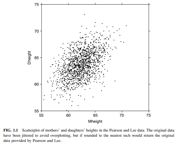
One of the first uses of regression was to study inheritance of traits from generation to generation. During the period 1893-1898, E. S. Pearson organized the collection of $n=1375$ heights of mothers in the United Kingdom under the age of 65 and one of their adult daughters over the age of 18. Pearson and Lee (1903) published the data, and we shall use these data to examine inheritance. The data are given in the data file heights. txt $^1$.
Our interest is in inheritance from the mother to the daughter, so we view the mother’s height, called Mheight, as the predictor variable and the daughter’s height, Dheight, as the response variable. Do taller mothers tend to have taller daughters? Do shorter mothers tend to have shorter daughters?
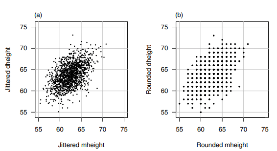
A scatterplot of Dheight versus Mheight helps us answer these questions. The scatterplot is a graph of each of the $n$ points with the response Dheight on the vertical axis and predictor Mheight on the horizontal axis. This plot is shown in Figure 1.1. For regression problems with one predictor $X$ and a response $Y$, we call the scatterplot of $Y$ versus $X$ a summary graph.
Here are some important characteristics of Figure 1.1:
The range of heights appears to be about the same for mothers and for daughters. Because of this, we draw the plot so that the lengths of the horizontal and vertical axes are the same, and the scales are the same. If all mothers and daughters had exactly the same height, then all the points would fall exactly on a $45^{\circ}$ line. Some computer programs for drawing a scatterplot are not smart enough to figure out that the lengths of the axes should be the same, so you might need to resize the plot or to draw it several times.
The original data that went into this scatterplot was rounded so each of the heights was given to the nearest inch. If we were to plot the original data, we would have substantial overplotting with many points at exactly the same location. This is undesirable because we will not know if one point represents one case or many cases, and this can be very misleading. The easiest solution is to use jittering, in which a small uniform random number is added to each value. In Figure 1.1, we used a uniform random number on the range from -0.5 to +0.5 , so the jittered values would round to the numbers given in the original source.
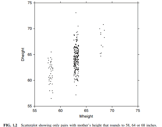
One important function of the scatterplot is to decide if we might reasonably assume that the response on the vertical axis is independent of the predictoron the horizontal axis. This is clearly not the case here since as we move across Figure 1.1 from left to right, the scatter of points is different for each value of the predictor. What we mean by this is shown in Figure 1.2, in which we show only points corresponding to mother-daughter pairs with Mheight rounding to either 58,64 or 68 inches. We see that within each of these three strips or slices, even though the number of points is different within each slice, (a) the mean of Dheight is increasing from left to right, and (b) the vertical variability in Dheight seems to be more or less the same for each of the fixed values of Mheight.
The scatter of points in the graph appears to be more or less elliptically shaped, with the axis of the ellipse tilted upward. We will see in Section 4.3 that summary graphs that look like this one suggest use of the simple linear regression model that will be discussed in Chapter 2.
Scatterplots are also important for finding separated points, which are either points with values on the horizontal axis that are well separated from the other points or points with values on the vertical axis that, given the value on the horizontal axis, are either much too large or too small. In terms of this example, this would mean looking for very tall or short mothers or, alternatively, for daughters who are very tall or short, given the height of their mother.
统计代写|线性回归代写Linear Regression代考|Forbes’ Data
In an 1857 article, a Scottish physicist named James D. Forbes discussed a series of experiments that he had done concerning the relationship between atmospheric pressure and the boiling point of water. He knew that altitude could be determined from atmospheric pressure, measured with a barometer, with lower pressures corresponding to higher altitudes. In the middle of the nineteenth century, barometers were fragile instruments, and Forbes wondered if a simpler measurement of the boiling point of water could substitute for a direct reading of barometric pressure. Forbes collected data in the Alps and in Scotland. He measured at each location pressure in inches of mercury with a barometer and boiling point in degrees Fahrenheit using a thermometer. Boiling point measurements were adjusted for the difference between the ambient air temperature when he took the measurements and a standard temperature. The data for $n=17$ locales are reproduced in the file forbes.txt.
The scatterplot of Pressure versus Temp is shown in Figure 1.3a. The general appearance of this plot is very different from the summary graph for the heights data. First, the sample size is only 17, as compared to over 1300 for the heights data. Second, apart from one point, all the points fall almost exactly on a smooth curve. This means that the variability in pressure for a given temperature is extremely small.
The points in Figure 1.3a appear to fall very close to the straight line shown on the plot, and so we might be encouraged to think that the mean of pressure given temperature could be modelled by a straight line. Look closely at the graph, and you will see that there is a small systematic error with the straight line: apart from the one point that does not fit at all, the points in the middle of the graph fall below the line, and those at the highest and lowest temperatures fall above the line. This is much easier to see in Figure $1.3 \mathrm{~b}$, which is obtained by removing the linear trend from Figure 1.3a, so the plotted points on the vertical axis are given for each value of Temp by
Residual $=$ Pressure – point on the line
This allows us to gain resolution in the plot since the range on the vertical axis in Figure $1.3 \mathrm{a}$ is about 10 inches of mercury while the range in Figure $1.3 \mathrm{~b}$ is about 0.8 inches of mercury. To get the same resolution in Figure 1.3a, we would need a graph that is $10 / 0.8=12.5$ as big as Figure 1.3b. Again ignoring the one point that clearly does not match the others, the curvature in the plot is clearly visible in Figure 1.3b.
线性回归代写
统计代写|线性回归代写Linear Regression代考|SCATTERPLOTS
我们从一个回归问题开始,有一个预测器,我们通常称之为X,一个响应变量,我们称之为Y。数据由$\left(x_i, y_i\right), i=1, \ldots, n$, $(X, Y)$在$n$个单位或案例中观察到的值组成。在任何特定问题中,$X$和$Y$都有其他名称,如温度或浓度,这些名称更能描述要分析的数据。回归的目标是理解$Y$的值如何随着$X$在其可能值范围内的变化而变化。从散点图中可以首先看到$Y$随着$X$的变化是如何变化的。
身高的遗传
回归的最初用途之一是研究性状的遗传代代相传。1893-1898年,E. S. Pearson收集了英国65岁以下的母亲和一个18岁以上的成年女儿的$n=1375$身高。Pearson和Lee(1903)发表了这些数据,我们将使用这些数据来检验遗传。数据在数据文件高度中给出。txt ^ 1美元。
我们感兴趣的是从母亲到女儿的遗传,因此我们将母亲的身高(称为Mheight)视为预测变量,将女儿的身高(称为Dheight)视为响应变量。更高的母亲会生出更高的女儿吗?矮一些的母亲会生出矮一些的女儿吗?
Dheight和Mheight的散点图可以帮助我们回答这些问题。散点图是每个$n$点的图形,纵轴表示响应Dheight,横轴表示预测器Mheight。该图如图1.1所示。对于有一个预测因子X$和一个响应因子Y$的回归问题,我们称Y$和X$的散点图为汇总图。以下是图1.1的一些重要特征:
母亲和女儿的身高范围似乎大致相同。正因为如此,我们绘制的图使水平轴和垂直轴的长度相同,并且比例尺相同。如果所有的母亲和女儿有完全相同的高度,那么所有的点将完全落在$45^{\circ}$线上。一些用于绘制散点图的计算机程序不够聪明,无法计算出轴的长度应该是相同的,因此您可能需要调整图的大小或多次绘制它。
进入这个散点图的原始数据是四舍五入的,所以每个高度都给出了最近的英寸。如果我们要绘制原始数据,我们将在完全相同的位置上绘制大量的重叠点。这是不可取的,因为我们不知道是一个点代表一个情况还是许多情况,这可能会非常误导。最简单的解决方案是使用抖动,其中每个值添加一个小的均匀随机数。在图1.1中,我们在-0.5到+0.5的范围内使用了一个统一的随机数,因此抖动值将四舍五入到原始源中给出的数字。
散点图的一个重要功能是决定我们是否可以合理地假设纵轴上的响应与横轴上的预测无关。这显然不是这里的情况,因为当我们从左向右移动图1.1时,预测器的每个值的点的分散是不同的。图1.2显示了我们的意思,其中我们只显示了对应于母女对的点,其中Mheight四舍五入为58、64或68英寸。我们看到,在这三条或切片中的每一条中,尽管每个切片中的点数不同,(a) Dheight的平均值从左到右增加,(b)对于每个固定的Mheight值,Dheight的垂直变化似乎或多或少是相同的。
图中点的散点看起来或多或少呈椭圆形,椭圆轴向上倾斜。我们将在第4.3节中看到,类似这样的汇总图表明使用将在第2章中讨论的简单线性回归模型。
散点图对于寻找分离点也很重要,这些点要么是水平轴上的值与其他点分开得很好,要么是垂直轴上的值,给定水平轴上的值,要么太大要么太小。在这个例子中,这意味着寻找非常高或矮的母亲,或者,根据母亲的身高,寻找非常高或矮的女儿。
统计代写|线性回归代写Linear Regression代考|Forbes’ Data
在1857年的一篇文章中,一位名叫詹姆斯·d·福布斯的苏格兰物理学家讨论了他所做的一系列关于大气压力和水沸点之间关系的实验。他知道海拔高度可以通过气压来确定,用气压计测量,气压越低海拔越高。在19世纪中叶,气压计是一种易碎的仪器,福布斯想知道是否可以用一种更简单的测量水沸点的方法来代替直接读数气压计。福布斯在阿尔卑斯山和苏格兰收集数据。他用气压计测量每个地点的压力,单位是英寸汞柱,用温度计测量沸点,单位是华氏度。沸点测量是根据测量时周围空气温度与标准温度之间的差异进行调整的。$n=17$ locale的数据在forbes.txt文件中复制。
压力与温度的散点图如图1.3a所示。该图的总体外观与高度数据的汇总图非常不同。首先,样本大小只有17个,而高度数据则超过1300个。其次,除了一个点之外,所有的点几乎完全落在一条光滑的曲线上。这意味着在给定温度下压力的变化是极小的。
图1.3a中的点似乎非常接近图中所示的直线,因此我们可能会受到鼓舞,认为给定温度的压力平均值可以用一条直线来建模。仔细观察这张图,你会发现这条直线有一个小的系统误差:除了一个完全不适合的点外,图中中间的点都落在这条线以下,而温度最高和最低的点都落在这条线以上。这在图$1.3 \ mathm {~b}$中更容易看到,它是通过从图1.3a中删除线性趋势而得到的,因此垂直轴上的绘制点是为每个Temp by的值给出的
残余$=$管道上的压力点
这使我们能够在图中获得分辨率,因为图$1.3 \ mathm {a}$中垂直轴上的范围约为10英寸汞柱,而图$1.3 \ mathm {~b}$中的范围约为0.8英寸汞柱。为了获得与图1.3a相同的分辨率,我们需要一个与图1.3b一样大的10美元/ 0.8美元=12.5美元的图表。再次忽略一个明显与其他点不匹配的点,图1.3b中的曲度清晰可见。

统计代写|线性回归代写Linear Regression代考 请认准UprivateTA™. UprivateTA™为您的留学生涯保驾护航。
微观经济学代写
微观经济学是主流经济学的一个分支,研究个人和企业在做出有关稀缺资源分配的决策时的行为以及这些个人和企业之间的相互作用。my-assignmentexpert™ 为您的留学生涯保驾护航 在数学Mathematics作业代写方面已经树立了自己的口碑, 保证靠谱, 高质且原创的数学Mathematics代写服务。我们的专家在图论代写Graph Theory代写方面经验极为丰富,各种图论代写Graph Theory相关的作业也就用不着 说。
线性代数代写
线性代数是数学的一个分支,涉及线性方程,如:线性图,如:以及它们在向量空间和通过矩阵的表示。线性代数是几乎所有数学领域的核心。
博弈论代写
现代博弈论始于约翰-冯-诺伊曼(John von Neumann)提出的两人零和博弈中的混合策略均衡的观点及其证明。冯-诺依曼的原始证明使用了关于连续映射到紧凑凸集的布劳威尔定点定理,这成为博弈论和数学经济学的标准方法。在他的论文之后,1944年,他与奥斯卡-莫根斯特恩(Oskar Morgenstern)共同撰写了《游戏和经济行为理论》一书,该书考虑了几个参与者的合作游戏。这本书的第二版提供了预期效用的公理理论,使数理统计学家和经济学家能够处理不确定性下的决策。
微积分代写
微积分,最初被称为无穷小微积分或 “无穷小的微积分”,是对连续变化的数学研究,就像几何学是对形状的研究,而代数是对算术运算的概括研究一样。
它有两个主要分支,微分和积分;微分涉及瞬时变化率和曲线的斜率,而积分涉及数量的累积,以及曲线下或曲线之间的面积。这两个分支通过微积分的基本定理相互联系,它们利用了无限序列和无限级数收敛到一个明确定义的极限的基本概念 。
计量经济学代写
什么是计量经济学?
计量经济学是统计学和数学模型的定量应用,使用数据来发展理论或测试经济学中的现有假设,并根据历史数据预测未来趋势。它对现实世界的数据进行统计试验,然后将结果与被测试的理论进行比较和对比。
根据你是对测试现有理论感兴趣,还是对利用现有数据在这些观察的基础上提出新的假设感兴趣,计量经济学可以细分为两大类:理论和应用。那些经常从事这种实践的人通常被称为计量经济学家。
Matlab代写
MATLAB 是一种用于技术计算的高性能语言。它将计算、可视化和编程集成在一个易于使用的环境中,其中问题和解决方案以熟悉的数学符号表示。典型用途包括:数学和计算算法开发建模、仿真和原型制作数据分析、探索和可视化科学和工程图形应用程序开发,包括图形用户界面构建MATLAB 是一个交互式系统,其基本数据元素是一个不需要维度的数组。这使您可以解决许多技术计算问题,尤其是那些具有矩阵和向量公式的问题,而只需用 C 或 Fortran 等标量非交互式语言编写程序所需的时间的一小部分。MATLAB 名称代表矩阵实验室。MATLAB 最初的编写目的是提供对由 LINPACK 和 EISPACK 项目开发的矩阵软件的轻松访问,这两个项目共同代表了矩阵计算软件的最新技术。MATLAB 经过多年的发展,得到了许多用户的投入。在大学环境中,它是数学、工程和科学入门和高级课程的标准教学工具。在工业领域,MATLAB 是高效研究、开发和分析的首选工具。MATLAB 具有一系列称为工具箱的特定于应用程序的解决方案。对于大多数 MATLAB 用户来说非常重要,工具箱允许您学习和应用专业技术。工具箱是 MATLAB 函数(M 文件)的综合集合,可扩展 MATLAB 环境以解决特定类别的问题。可用工具箱的领域包括信号处理、控制系统、神经网络、模糊逻辑、小波、仿真等。