如果你也在 怎样代写回归分析Regression Analysis 这个学科遇到相关的难题,请随时右上角联系我们的24/7代写客服。回归分析Regression Analysis被广泛用于预测和预报,其使用与机器学习领域有很大的重叠。在某些情况下,回归分析可以用来推断自变量和因变量之间的因果关系。重要的是,回归本身只揭示了固定数据集中因变量和自变量集合之间的关系。为了分别使用回归进行预测或推断因果关系,研究者必须仔细论证为什么现有的关系对新的环境具有预测能力,或者为什么两个变量之间的关系具有因果解释。当研究者希望使用观察数据来估计因果关系时,后者尤其重要。
回归分析Regression Analysis在统计建模中,回归分析是一组统计过程,用于估计因变量(通常称为 “结果 “或 “响应 “变量,或机器学习术语中的 “标签”)与一个或多个自变量(通常称为 “预测因子”、”协变量”、”解释变量 “或 “特征”)之间的关系。回归分析最常见的形式是线性回归,即根据特定的数学标准找到最适合数据的直线(或更复杂的线性组合)。例如,普通最小二乘法计算唯一的直线(或超平面),使真实数据与该直线(或超平面)之间的平方差之和最小。由于特定的数学原因(见线性回归),这使得研究者能够在自变量具有一组给定值时估计因变量的条件期望值(或人口平均值)。不太常见的回归形式使用稍微不同的程序来估计替代位置参数(例如,量化回归或必要条件分析),或在更广泛的非线性模型集合中估计条件期望值(例如,非参数回归)。
回归分析Regression Analysis代写,免费提交作业要求, 满意后付款,成绩80\%以下全额退款,安全省心无顾虑。专业硕 博写手团队,所有订单可靠准时,保证 100% 原创。 最高质量的回归分析Regression Analysis作业代写,服务覆盖北美、欧洲、澳洲等 国家。 在代写价格方面,考虑到同学们的经济条件,在保障代写质量的前提下,我们为客户提供最合理的价格。 由于作业种类很多,同时其中的大部分作业在字数上都没有具体要求,因此回归分析Regression Analysis作业代写的价格不固定。通常在专家查看完作业要求之后会给出报价。作业难度和截止日期对价格也有很大的影响。
同学们在留学期间,都对各式各样的作业考试很是头疼,如果你无从下手,不如考虑my-assignmentexpert™!
my-assignmentexpert™提供最专业的一站式服务:Essay代写,Dissertation代写,Assignment代写,Paper代写,Proposal代写,Proposal代写,Literature Review代写,Online Course,Exam代考等等。my-assignmentexpert™专注为留学生提供Essay代写服务,拥有各个专业的博硕教师团队帮您代写,免费修改及辅导,保证成果完成的效率和质量。同时有多家检测平台帐号,包括Turnitin高级账户,检测论文不会留痕,写好后检测修改,放心可靠,经得起任何考验!
想知道您作业确定的价格吗? 免费下单以相关学科的专家能了解具体的要求之后在1-3个小时就提出价格。专家的 报价比上列的价格能便宜好几倍。
我们在统计Statistics代写方面已经树立了自己的口碑, 保证靠谱, 高质且原创的统计Statistics代写服务。我们的专家在回归分析Regression Analysis代写方面经验极为丰富,各种回归分析Regression Analysis相关的作业也就用不着 说。
统计代写|回归分析代写Regression Analysis代考|Another Curve Fitting Example
Let’s go through one more example using both linear and nonlinear regression. As usual, our goal is to develop an unbiased model. These data are freely available from the NIST and pertain to the relationship between density and electron mobility. Download the CSV data file to try it yourself: ElectronMobility.
Linear model
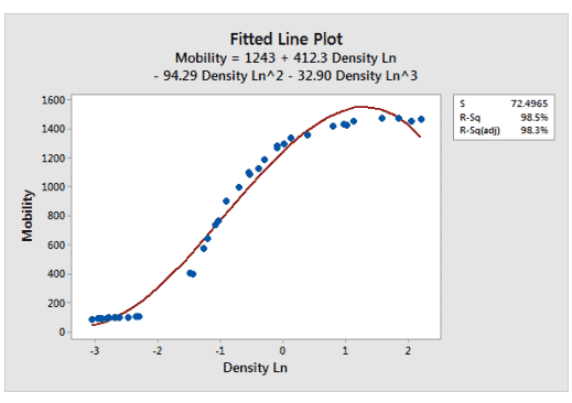
First, I’ll attempt to fit the curve using a linear model. Because there is only one independent variable, I can use a fitted line plot. In this model, I use a cubed term to fit the curvature because there are two bends.
The fitted relationship in the graph follows the data fairly close and produces a high R-squared of $98.5 \%$. Those sound great, but look more closely and you’ll notice that various places along the regression line consistently under and over-predict the observed values. This model is biased, and it again illustrates a point that I make in the chapter about goodness-of-fit. By themselves, high R-squared values don’t necessarily indicate that you have a good model.
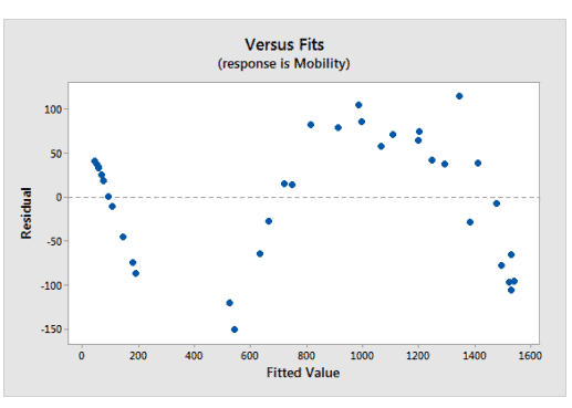
Because we have only one independent variable, we can plot the relationship on the fitted line plot. However, when you have more than one independent variable, you can’t use a fitted line plot and you’ll need to rely on residual plots to check the regression assumptions. For our data, the residual plots display the nonrandom patterns very clearly. You want to see random residuals.
Our linear regression model can’t adequately fit the curve in the data. There’s nothing more we can do with linear regression. Consequently, it’s time to try nonlinear regression.
Example of a nonlinear regression model
Now, let’s fit the same data but using nonlinear regression. As I mentioned earlier, nonlinear regression can be harder to perform. The fact that you can fit nonlinear models with virtually an infinite number of functional forms is both its strength and downside.
The main positive is that nonlinear regression provides the most flexible curve-fitting functionality. The downside is that it can take considerable effort to choose the nonlinear function that creates the best fit for the particular shape of the curve. Unlike linear regression, you also need to supply starting values for the nonlinear algorithm. Some datasets can require substantial effort to find acceptable starting values. For instance, some starting values can cause the algorithm to fail to converge on a solution or to converge on an incorrect solution. It’s for these reasons that I always recommend fitting linear models first.
Our example dataset is one that the NIST uses to illustrate a hard-tofit nonlinear relationship. So, it’s no surprise that the linear model was insufficient. Because this section focuses on the basics of choosing between linear and nonlinear models, I’m not going to cover how the researchers chose the optimal functional form of the nonlinear model.
统计代写|回归分析代写Regression Analysis代考|Review and Next Steps
In the fitted line plot, the nonlinear relationship follows the data almost exactly. The residual plot displays the randomness that we want to see for an unbiased model. R-squared does not appear because it is invalid for nonlinear regression. However, we can compare the standard error of the regression (S) for the two models. You want $\mathrm{S}$ to be smaller because it indicates that the data points are closer to the fitted line. For the linear model, $\mathrm{S}$ is 72.5 while for the nonlinear model it is 13.7. The nonlinear model provides a better fit because it is both unbiased and produces smaller residuals.
Nonlinear regression is a powerful alternative to linear regression but there are a few drawbacks. Fortunately, it’s not difficult to try linear regression first.
Curvature happens when the effect of an independent variable varies based on its own value. It’s easiest to detect curved relationships by plotting your data on scatterplots. You can try a variety of methods to fit curvature, including the following:
- Polynomials in linear regression.
- Inverses in linear regression.
- Logs in linear regression.
- Nonlinear regression.
Use main effects plots to see how your model fits the curvature. Use fitted line plots, residual plots, and goodness-of-fit statistics, such as R-squared and S, to determine how well it fits the data. Collectively, these tools help you decide which approach is best for your data.
Don’t rely solely on the goodness-of-fit statistics because even an excellent value doesn’t necessarily mean that you fit the curvature adequately. Use statistical measures in conjunction with graphs!
Next, I’ll cover interaction effects, which occur when the effect of one independent variable depends on the value of a different independent variable.
回归分析代写
统计代写|回归分析代写REGRESSION ANALYSIS代考|ANOTHER CURVE FITTING EXAMPLE
让我们再看一个使用线性和非线性回归的例子。像往常一样,我们的目标是开发一个无偏见的模型。这些数据可从 NIST 免费获得,并且与密度和电子迁移率之间的关系有关。下载 CSV 数据文件亲自尝试:ElectronMobility。
线性模型
首先,我将尝试使用线性模型来拟合曲线。因为只有一个自变量,所以我可以使用拟合线图。在此模型中,我使用立方项来拟合曲率,因为有两个弯曲。
图中的拟合关系非常接近数据并产生高 R 平方
. 这些听起来不错,但仔细观察,您会注意到回归线上的各个位置始终低于和高于预测的观察值。这个模型是有偏见的,它再次说明了我在有关拟合优度的章节中提出的观点。就其本身而言,高 R 平方值并不一定表示您拥有一个好的模型。
因为我们只有一个自变量,所以我们可以在拟合线图上绘制关系。但是,当您有多个自变量时,您不能使用拟合线图,您需要依靠残差图来检查回归假设。对于我们的数据,残差图非常清楚地显示了非随机模式。你想看到随机残差。
我们的线性回归模型无法充分拟合数据中的曲线。对于线性回归,我们无能为力。因此,是时候尝试非线性回归了。
非线性回归模型示例
现在,让我们拟合相同的数据,但使用非线性回归。正如我之前提到的,非线性回归可能更难执行。您可以用几乎无限数量的函数形式来拟合非线性模型这一事实既是它的优点也是缺点。
主要的好处是非线性回归提供了最灵活的曲线拟合功能。不利之处在于,选择最适合特定曲线形状的非线性函数可能需要付出相当大的努力。与线性回归不同,您还需要为非线性算法提供起始值。某些数据集可能需要付出大量努力才能找到可接受的起始值。例如,某些起始值可能导致算法无法收敛于一个解或收敛于一个不正确的解。出于这些原因,我总是建议首先拟合线性模型。
我们的示例数据集是 NIST 用来说明难以拟合的非线性关系的数据集。因此,线性模型不足也就不足为奇了。由于本节重点介绍在线性模型和非线性模型之间进行选择的基础知识,因此我不会介绍研究人员如何选择非线性模型的最佳函数形式。
统计代写|回归分析代写REGRESSION ANALYSIS代考|REVIEW AND NEXT STEPS
在拟合线图中,非线性关系几乎完全符合数据。残差图显示了我们希望看到的无偏模型的随机性。R-squared 没有出现,因为它对非线性回归无效。但是,我们可以比较回归的标准误差
对于这两个模型。你要
更小,因为它表明数据点更接近拟合线。对于线性模型,
是 72.5,而非线性模型是 13.7。非线性模型提供更好的拟合,因为它既无偏又产生较小的残差。
非线性回归是线性回归的有力替代方法,但也有一些缺点。幸运的是,先尝试线性回归并不难。
当自变量的影响根据其自身的值而变化时,就会发生曲率。通过在散点图上绘制数据最容易检测曲线关系。您可以尝试多种方法来拟合曲率,包括以下几种:
线性回归中的多项式。
线性回归中的逆。
登录线性回归。
非线性回归。
使用主效应图查看您的模型如何拟合曲率。使用拟合线图、残差图和拟合优度统计量(例如 R 平方和 S)来确定它与数据的拟合程度。这些工具共同帮助您决定哪种方法最适合您的数据。
不要仅仅依赖拟合优度统计数据,因为即使是极好的值也不一定意味着您可以充分拟合曲率。将统计措施与图表结合使用!
接下来,我将介绍交互作用,当一个自变量的影响取决于另一个自变量的值时会发生这种作用。

统计代写|回归分析代写Regression Analysis代考 请认准UprivateTA™. UprivateTA™为您的留学生涯保驾护航。
微观经济学代写
微观经济学是主流经济学的一个分支,研究个人和企业在做出有关稀缺资源分配的决策时的行为以及这些个人和企业之间的相互作用。my-assignmentexpert™ 为您的留学生涯保驾护航 在数学Mathematics作业代写方面已经树立了自己的口碑, 保证靠谱, 高质且原创的数学Mathematics代写服务。我们的专家在图论代写Graph Theory代写方面经验极为丰富,各种图论代写Graph Theory相关的作业也就用不着 说。
线性代数代写
线性代数是数学的一个分支,涉及线性方程,如:线性图,如:以及它们在向量空间和通过矩阵的表示。线性代数是几乎所有数学领域的核心。
博弈论代写
现代博弈论始于约翰-冯-诺伊曼(John von Neumann)提出的两人零和博弈中的混合策略均衡的观点及其证明。冯-诺依曼的原始证明使用了关于连续映射到紧凑凸集的布劳威尔定点定理,这成为博弈论和数学经济学的标准方法。在他的论文之后,1944年,他与奥斯卡-莫根斯特恩(Oskar Morgenstern)共同撰写了《游戏和经济行为理论》一书,该书考虑了几个参与者的合作游戏。这本书的第二版提供了预期效用的公理理论,使数理统计学家和经济学家能够处理不确定性下的决策。
微积分代写
微积分,最初被称为无穷小微积分或 “无穷小的微积分”,是对连续变化的数学研究,就像几何学是对形状的研究,而代数是对算术运算的概括研究一样。
它有两个主要分支,微分和积分;微分涉及瞬时变化率和曲线的斜率,而积分涉及数量的累积,以及曲线下或曲线之间的面积。这两个分支通过微积分的基本定理相互联系,它们利用了无限序列和无限级数收敛到一个明确定义的极限的基本概念 。
计量经济学代写
什么是计量经济学?
计量经济学是统计学和数学模型的定量应用,使用数据来发展理论或测试经济学中的现有假设,并根据历史数据预测未来趋势。它对现实世界的数据进行统计试验,然后将结果与被测试的理论进行比较和对比。
根据你是对测试现有理论感兴趣,还是对利用现有数据在这些观察的基础上提出新的假设感兴趣,计量经济学可以细分为两大类:理论和应用。那些经常从事这种实践的人通常被称为计量经济学家。
Matlab代写
MATLAB 是一种用于技术计算的高性能语言。它将计算、可视化和编程集成在一个易于使用的环境中,其中问题和解决方案以熟悉的数学符号表示。典型用途包括:数学和计算算法开发建模、仿真和原型制作数据分析、探索和可视化科学和工程图形应用程序开发,包括图形用户界面构建MATLAB 是一个交互式系统,其基本数据元素是一个不需要维度的数组。这使您可以解决许多技术计算问题,尤其是那些具有矩阵和向量公式的问题,而只需用 C 或 Fortran 等标量非交互式语言编写程序所需的时间的一小部分。MATLAB 名称代表矩阵实验室。MATLAB 最初的编写目的是提供对由 LINPACK 和 EISPACK 项目开发的矩阵软件的轻松访问,这两个项目共同代表了矩阵计算软件的最新技术。MATLAB 经过多年的发展,得到了许多用户的投入。在大学环境中,它是数学、工程和科学入门和高级课程的标准教学工具。在工业领域,MATLAB 是高效研究、开发和分析的首选工具。MATLAB 具有一系列称为工具箱的特定于应用程序的解决方案。对于大多数 MATLAB 用户来说非常重要,工具箱允许您学习和应用专业技术。工具箱是 MATLAB 函数(M 文件)的综合集合,可扩展 MATLAB 环境以解决特定类别的问题。可用工具箱的领域包括信号处理、控制系统、神经网络、模糊逻辑、小波、仿真等。